At the beginning.
In the previous group meeting, I presented the results of quantifying pressure pulsations in planes and curved surfaces. My tutor hoped that I could teach this data post-processing method to everyone in the research group, so I wrote this article.
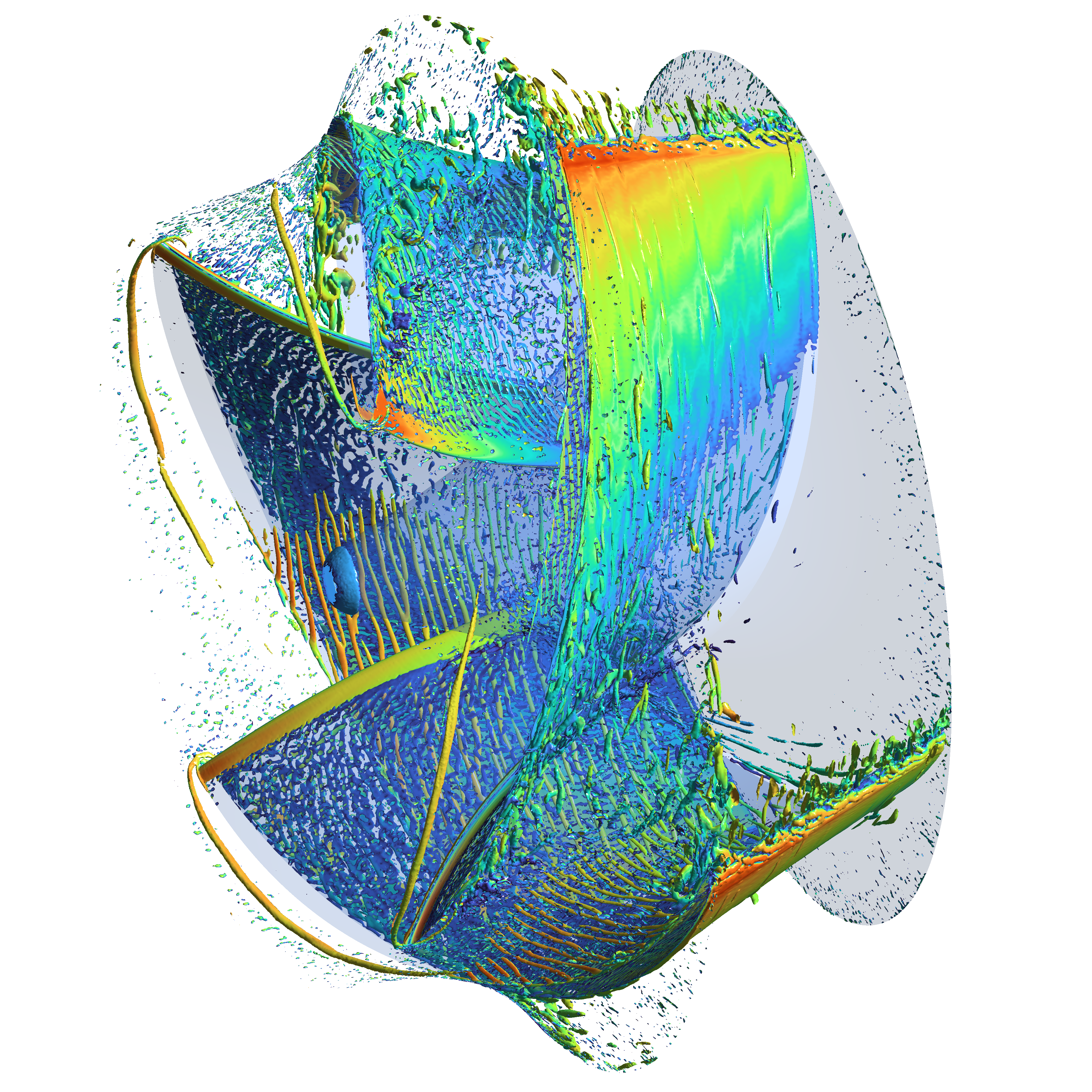
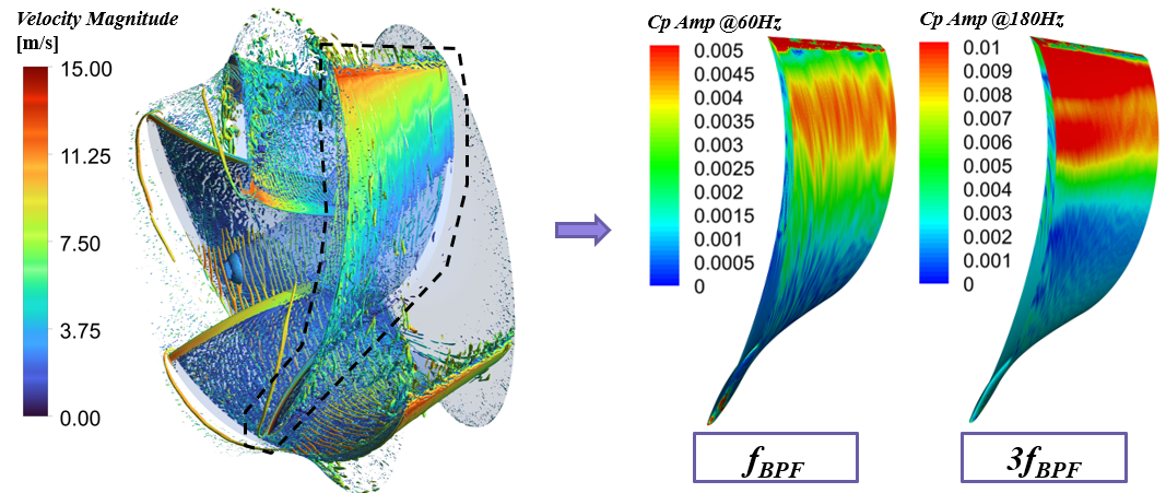
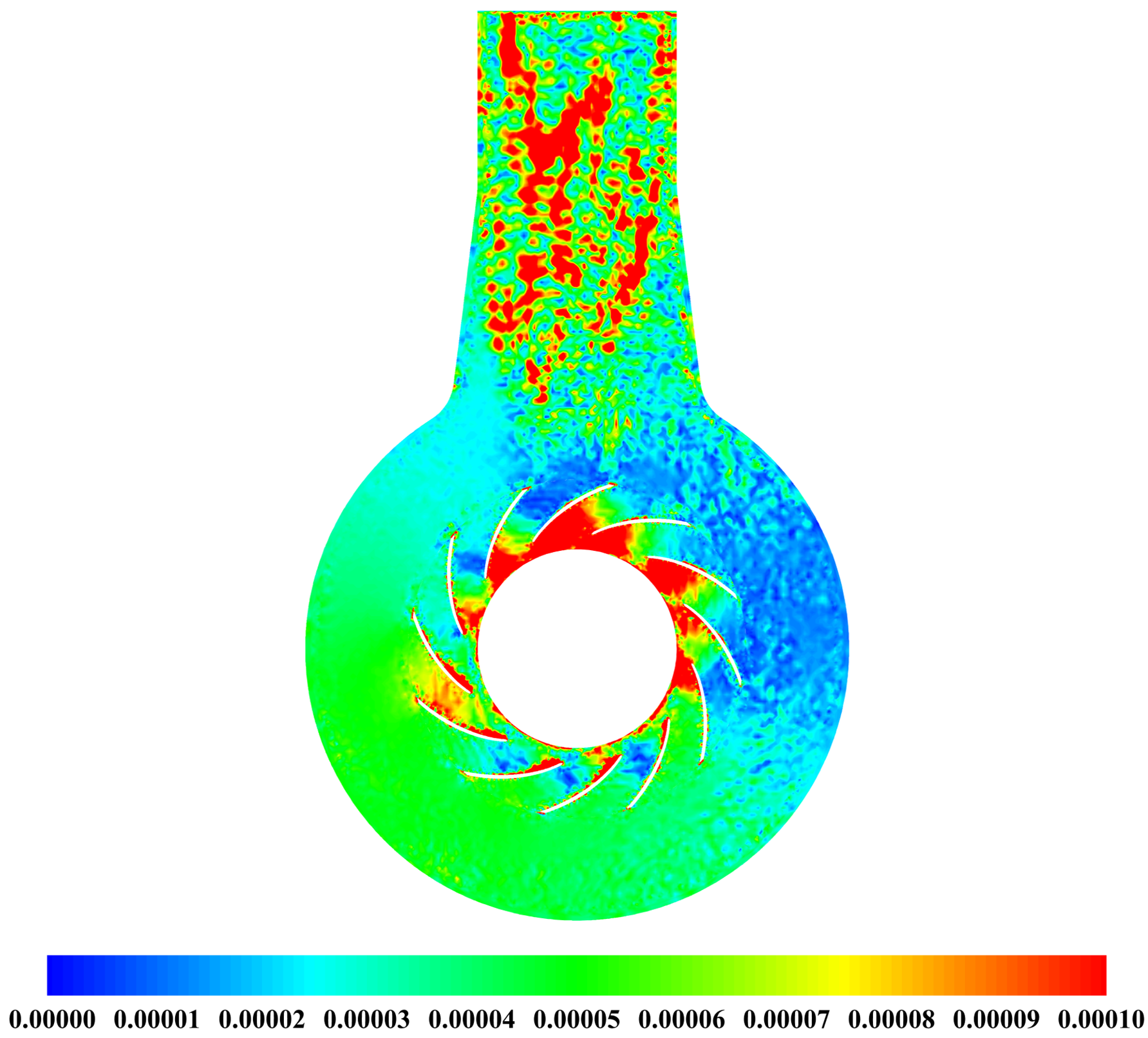
Although it is difficult to present a quantitative result for higher-dimensional pressure pulsation, it is a very intuitive method for qualitative research. For example, in the figure below, I used this method to process the pressure pulsation distributed on the surface of the mixed flow impeller blades, and the spatial distribution law of the pressure pulsation intensity at different frequencies can be clearly observed. This method may play an important role in the future blade design process.
In order to make this method feasible, we need to prepare the code we need to use before processing the data.
Adhering to the principle of "just work", the whole set of codes is written really bad in some places.💩💩
But if you follow this tutorial, everything will be fine.
What is High-dimensional FFT?
Since we want to get the pressure pulsation of a plane or a surface, we need to know how to get pressure information from the surface we want to deal with.High dimensional FFT is essentially consume every single mesh node on the surface we want to deal with as our monitoring point, which means we need to setup monitoring surface in Fluent first.
Step 1. Setup Monitoring Surface in Fluent
First, open Ansys Fluent with reading the case & data.
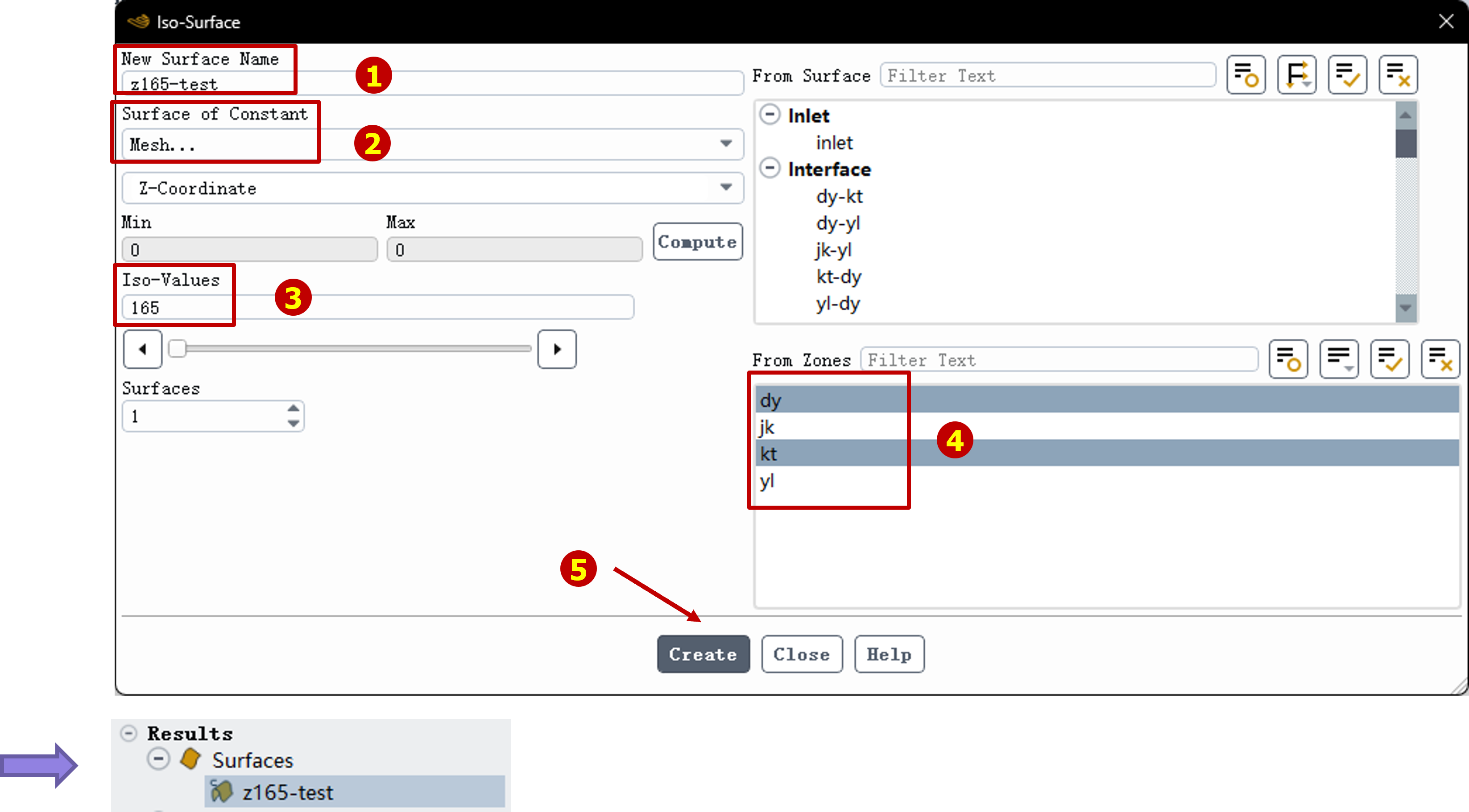
Then create the monitoring surface by following the steps illustrated in the picture below.
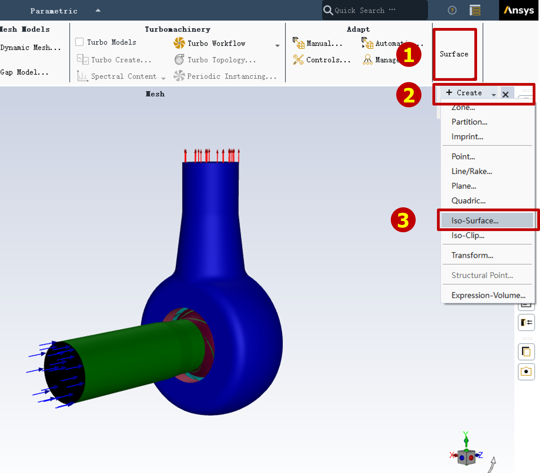
Type in the name and choose "Surface of Constant" into "Mesh".
Assuming the plane Z=165 is the surface we want, so we choose "Z-coordinate" and set the value as 165.
Also, we need to choose which flow domain can be cut by this plane. In this study, I would like to research how pressure pulctuating in the casing and guide vane, thus I need to choose "kt"(casing) and "dy"(guide vane). You can choose any other flow domain you want to research, too.
After doing this, you can find a new surface we just created under the surface tree.
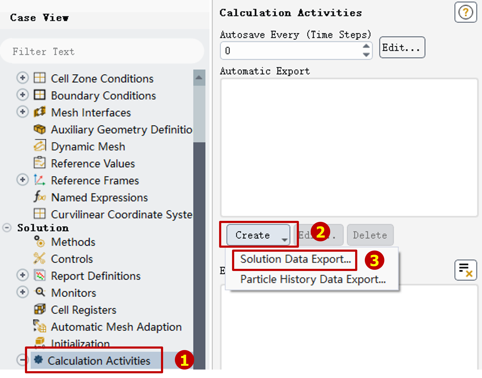
Then double click the "Calculation Activities" in the "Outline view", the "Task Page" will change.
Click the "Create" button then click "Solution Data Export" to set automatic data export.
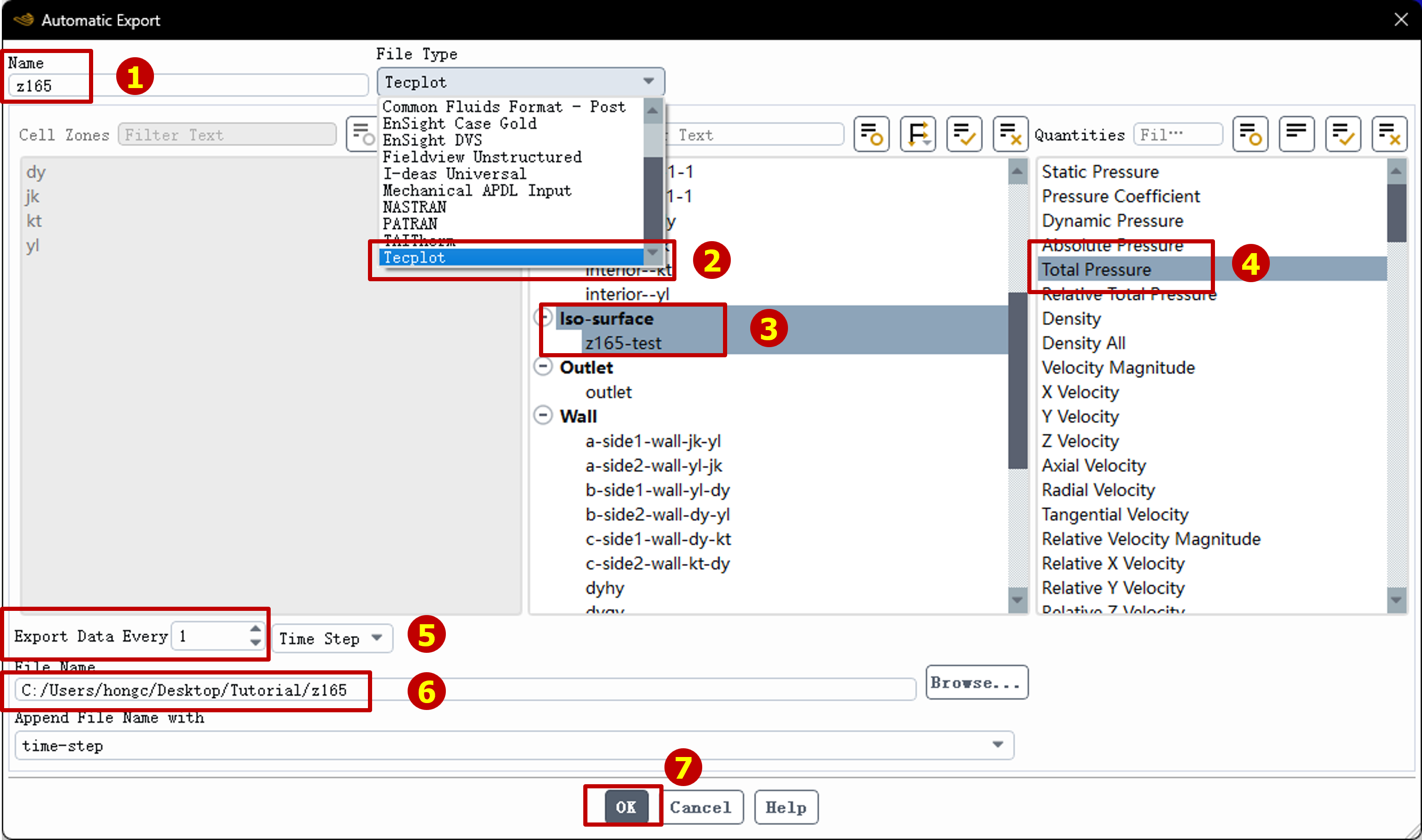
Change the name in the jumped-out window and select "File type" as "Tecplot" (Update 2025/12/11: If your data across multi computational domain, use CGNS format instead.), then select the Iso-surface we just created and select "Total Pressure" in the "Quantities".
Make sure it will export data every single time step(if you don't need such high sampling rate, you can alse change it into 2 or 3 time steps export once.)
Save data to the path easy to find then click "OK"
To now, you can start calculation and wait for the data.
Step 2. Convert Data Formation into *.dat
The formation of tecplot(*.plt) is encrypted which means we can't parse is directly, thus we need to do formation conversion to make plt files easy to read.
Here, we need Tecplot convert data into ASCII encoded files by using Tecplot script where you can download through this link.
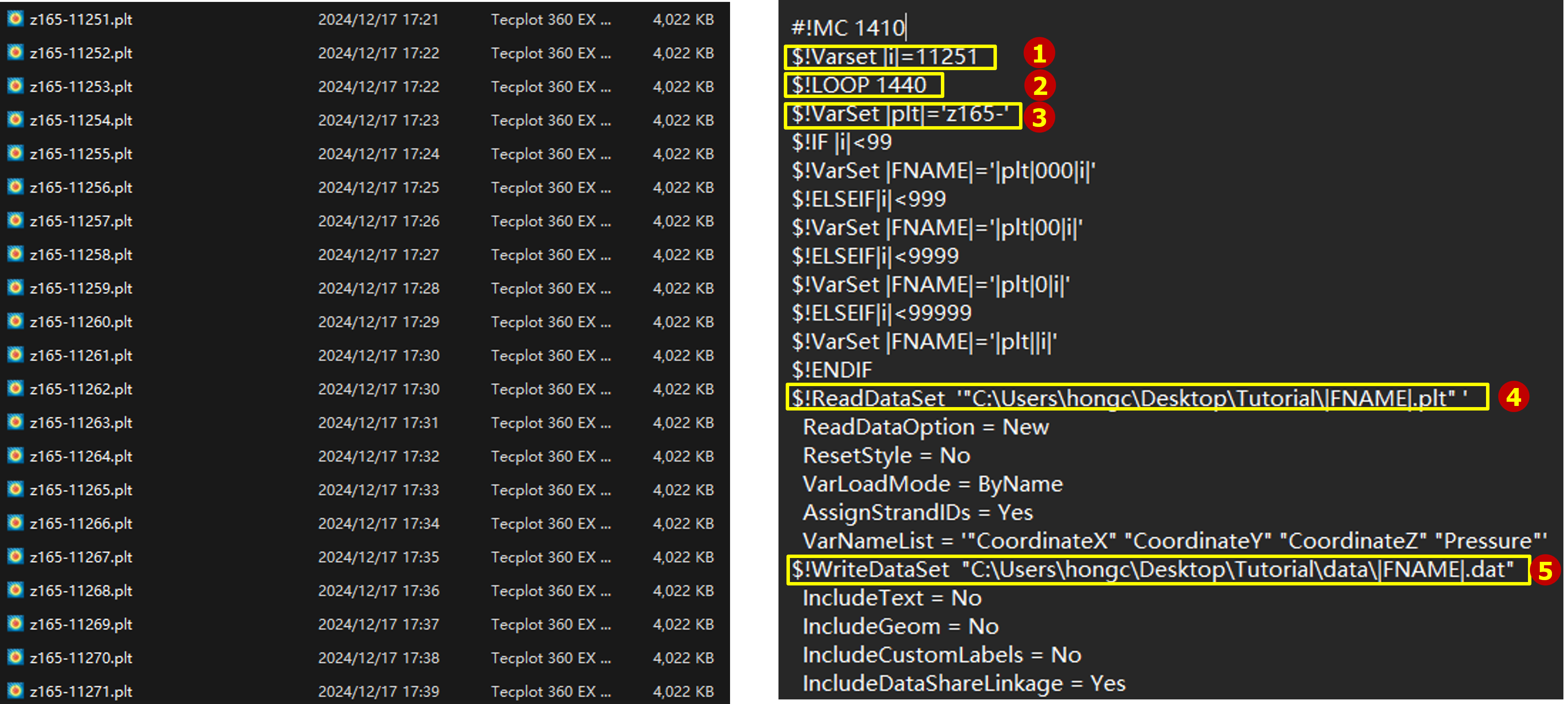
After calculation, we got tons of data files (1440 Time steps for example). But don't worry, every post-processing is automatic.
Open the Tecplot script file that you download from my website, you need to change several variables to fit your data.
As marked in the picture below, you need to modify the Start check mark "|i|". As you can see, our data are ordered by name, so we just change "|i|" as the number in the first file name.
And the "LOOP" number equals the number of our data files which is 1440 for example.
We also need to change the prefix in the script which should be "z165-". (Don't forget the dash "-")
In the end, change the read/write path. Create a new folder to hold new data is recommended.
Save the script file and open the Tecplot.
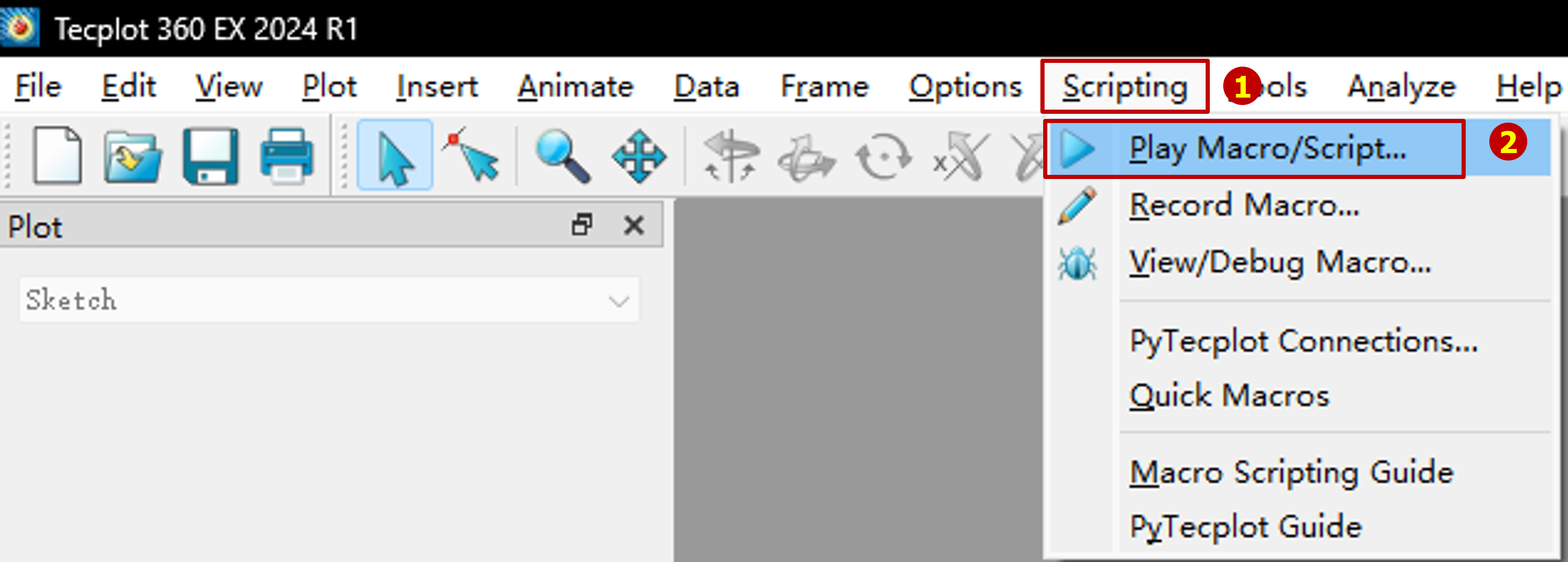
Select "Scripting" in the navigation bar above then click "Play Macro/Script" to play the script file we just modified.
Step 3. Open Matlab and Process the Data
After Step 2. we can get another 1440 data files ASCII encoded, so we can process the data by using Matlab.
Open code with Matlab.
There are a few things need to modify.
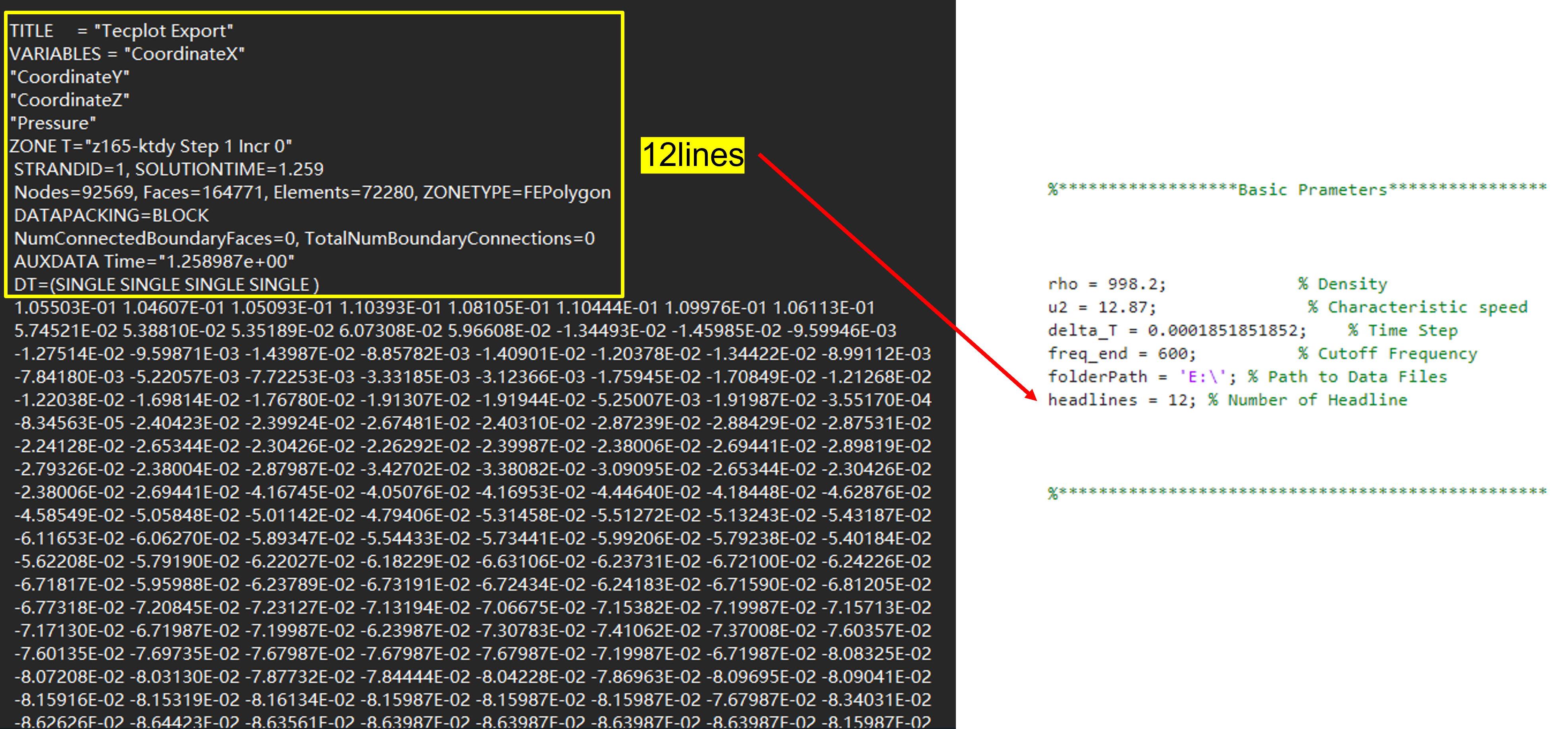
We can open the data file end with *.dat by using Notepad to observe the structure of it.
As illustrated in the picture below, we can easily find out that the first 12 lines are dicription lines which we need to skip. Thus the value of headlines should be 12 in this case.
Other parameters such as delta_T and u2 should be the same as it in fluent case.
Finish the steps above, press F5 to run this program.
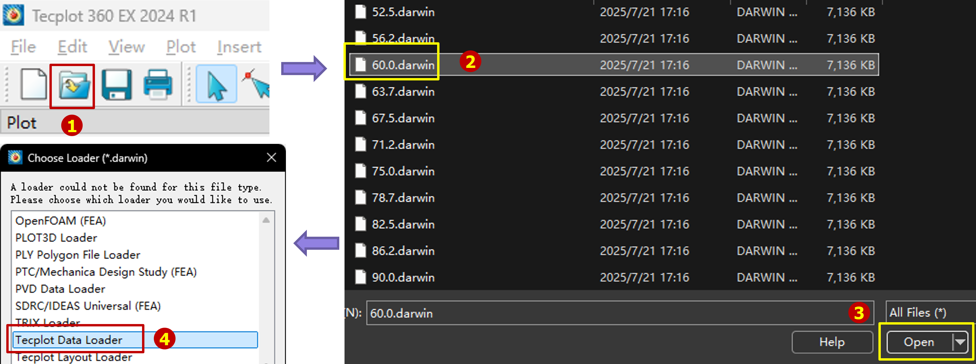
Wait for a wwhile, we can get bunch of files end with *.darwin, which can be opened by Tecplot.
Open Tecplot, click open data button and select the frequency you want to see.
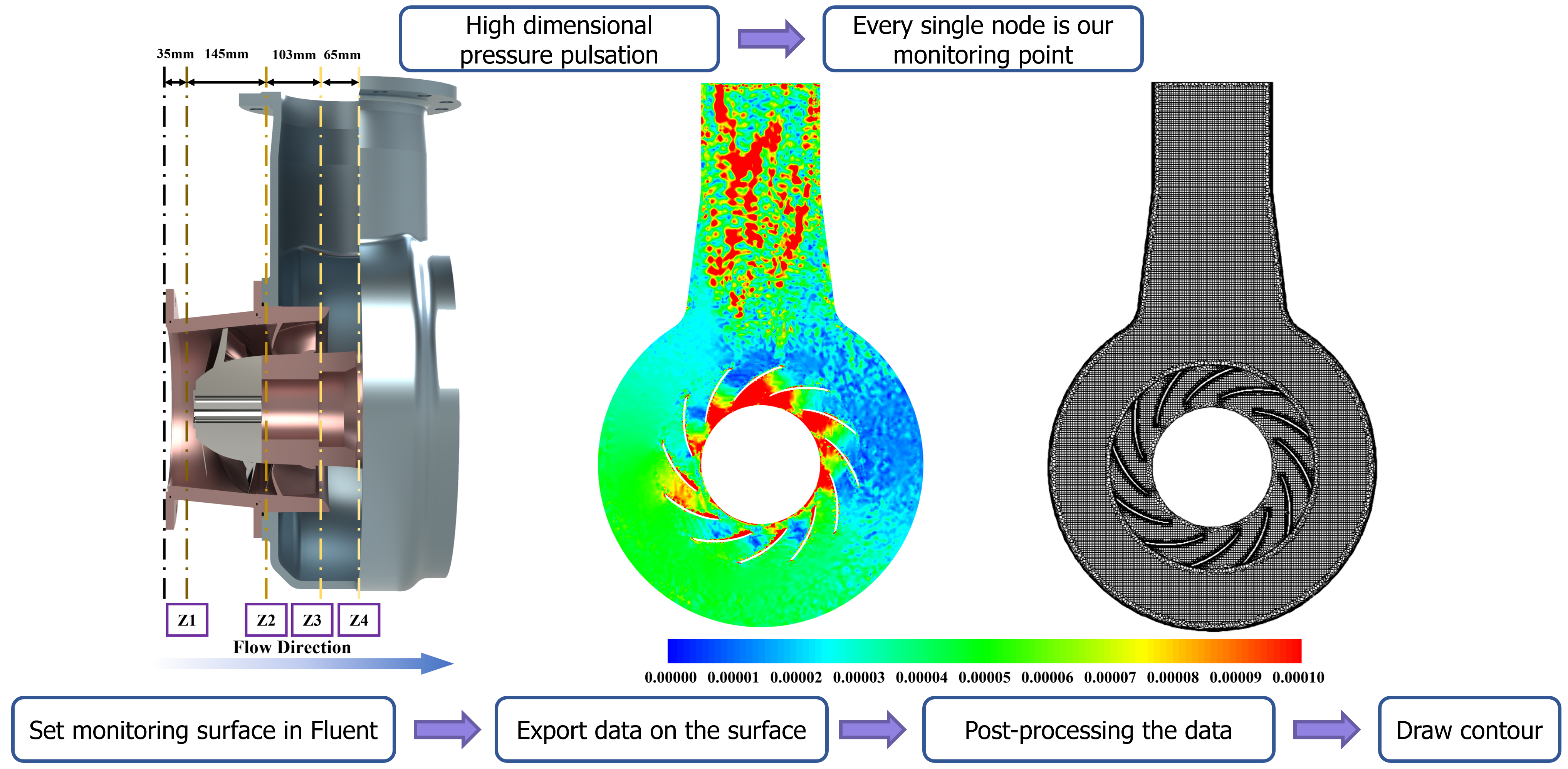
Then do some contour settings you can get the pressure pulsation contour of plane Z=165 like picture below.
The amplitude of the contour is dimension-less number Cp.
What's more?
By using this method you can not just only process the data on a plane, but also on a skewed surface such as blade surface like I showed at the beginning of the article.Also you can do research on fluctuation of voticity, every component of the velocity and turbulent kinetic energy and so on.
But here is one condition need to be aware, that is you have to ensure that the number of the mesh node remains constant which means you can't research impeller domain from the onlet direction. Because the number of the mesh node may change if you do so.