This document describes the basic workflow for generating an unstructured mesh using ANSYS ICEM CFD, and then performing steady-state simulation and post-processing in ANSYS Fluent. The workflow covers model import, geometry treatment, boundary naming, mesh generation, mesh export, Fluent steady-state setup, result saving, pump head and efficiency calculation, and contour post-processing in both Fluent and CFD-Post.

Note: Menu names and interface layouts may vary slightly among different ANSYS versions, but the overall workflow is generally the same. In practical applications, the settings should be adjusted according to the model structure, rotation direction, boundary conditions, and operating parameters.

1. Unstructured Meshing in ICEM

1.1 Open ICEM and Set the Working Directory

First, start ANSYS ICEM CFD. Before beginning the formal workflow, it is recommended to create a separate working folder for the current project. This folder should be used to store the geometry model, mesh files, and solver input/output files generated later. This avoids mixing files from different projects.

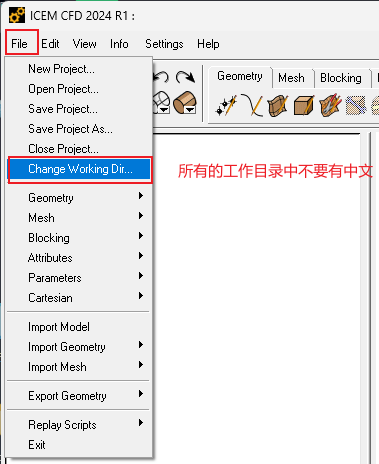
In ICEM, select:

File → Change Working Directory

Then select the corresponding working directory.

---

1.2 Import the Geometry Model

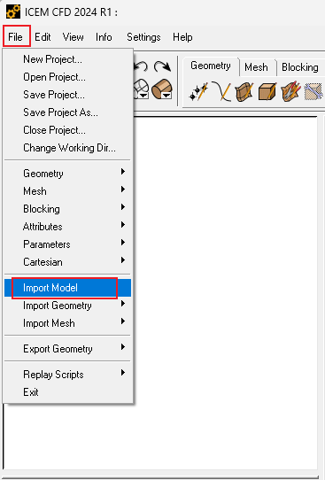
Select:

File → Import Model

Import the geometry model that needs to be meshed. Pay special attention to the unit setting during import. In this example, the unit is set to millimeter. If the actual geometry unit is inconsistent with the unit selected during import, the model scale in Fluent will be incorrect, which will affect the calculated flow rate, velocity, pump head, efficiency, and other results.

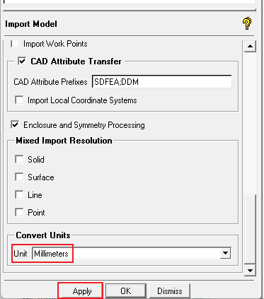
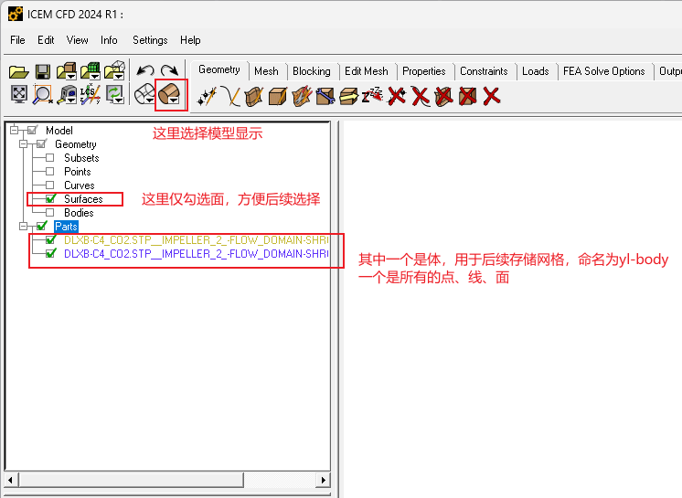
After importing the model, first check whether the complete model is displayed correctly and whether there are obvious missing faces, overlapping faces, or redundant bodies. If the geometry display is abnormal, repair the geometry in the original CAD software or directly in ICEM before proceeding.

---

1.3 Separate and Save the Visible Geometry

If the complete model contains multiple components, the parts that need to be meshed separately can be saved individually. The operation is as follows:

1. In the Parts tree on the left side, select the model part that needs to be retained.

2. Select:

   File → Geometry → Save Visible Geometry As
   

3. Enter a file name and save the file. It is recommended to use English letters or numbers in the file name and avoid Chinese characters, spaces, or special symbols, because these may cause reading or writing errors in later steps.

4. Repeat the above steps for the other components.

5. After finishing, select:

   File → Close Project
   

Alternatively, it is not necessary to save the visible geometry separately. You can directly delete unnecessary surfaces and bodies in the current model, keeping only the part that needs to be meshed. After completing all operations, close the file and save it with a new name when prompted. This method is simpler. If this method is used, you can skip directly to 1.5 Define Interfaces and Wall Boundaries.

---

1.4 Perform Geometry Topology Processing

If the model was saved as a separate geometry file in the previous step, reopen that file:

File → Geometry → Open Geometry

After the model is loaded, perform geometry topology processing. Select:

Geometry → Repair Geometry → Apply

Topology processing is used to identify and repair small gaps, duplicate edges, disconnected boundaries, and other geometry problems. This makes subsequent boundary naming and mesh generation more stable. For pump flow-passage models, after topology processing, pay special attention to the inlet, outlet, impeller interface, guide-vane interface, and other key regions to ensure that they are correctly identified.

---

1.5 Define Interfaces and Wall Boundaries

Before mesh generation, different boundaries need to be named. Boundary names will be transferred directly into Fluent, so clear and standardized English or pinyin names are recommended.

The basic operation is as follows:

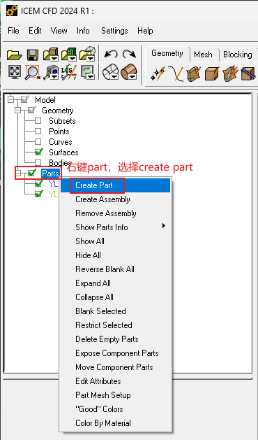
1. Right-click the Parts area in the upper-left panel and select:

   Create Part
   

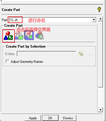
2. In the Part input box in the lower-left panel, enter the interface name, for example:

   yl-jk
   

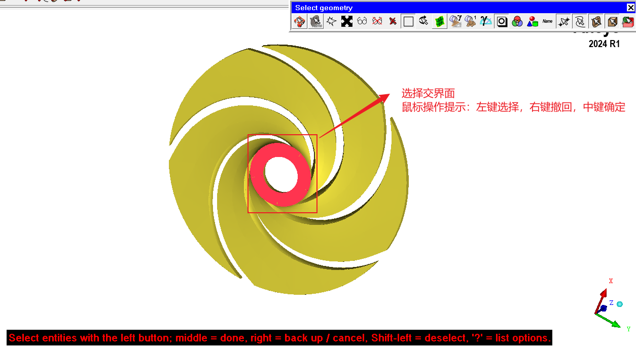
3. Select the corresponding interface surface.

4. Click Apply, or use the middle mouse button to confirm.

5. Use the same method to define other boundaries, such as inlet, outlet, interfaces, and periodic surfaces.

6. After all interface surfaces are defined, rename the remaining solid wall surfaces uniformly as:

   yl-wall
   

7. Finally, check whether all boundaries are completely and correctly named. Avoid undefined surfaces or incorrect boundary names.

Recommendation: Interface names should clearly distinguish connection surfaces between the rotating domain and the stationary domain, such as impeller inlet, impeller outlet, guide-vane inlet, and guide-vane outlet. Clear boundary names reduce the possibility of mistakes when defining mesh interfaces in Fluent.

---

1.6 Mesh Generation and Quality Check

After boundary naming is completed, the unstructured mesh can be generated.

1.6.1 Set the Global Mesh Size

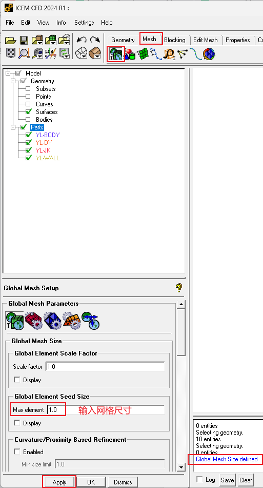
Select:

Mesh → Global Mesh Setup

In the Global Element Seed Size field in the lower-left panel, enter the global mesh size. For example:

3

Then click Apply.

The global mesh size is only a basic control parameter. Local refinement is usually required in regions such as the impeller, guide vanes, volute tongue, narrow gaps, and regions with strong curvature variation, depending on the required calculation accuracy.

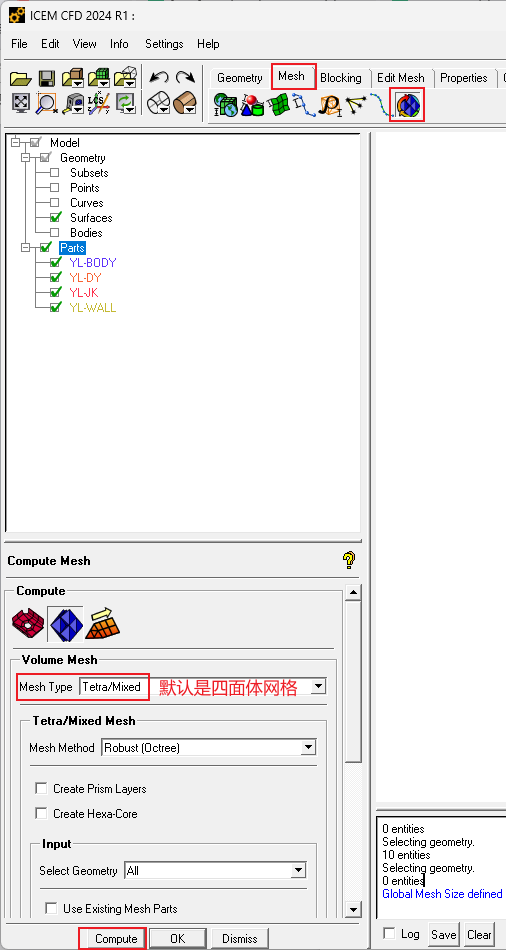
1.6.2 Generate the Mesh

Select:

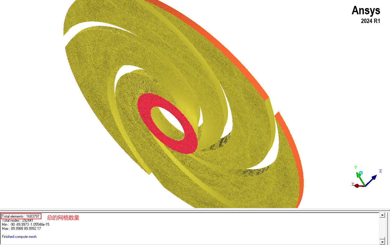
Mesh → Compute Mesh

Click Compute in the lower-left panel and wait until mesh generation is completed.

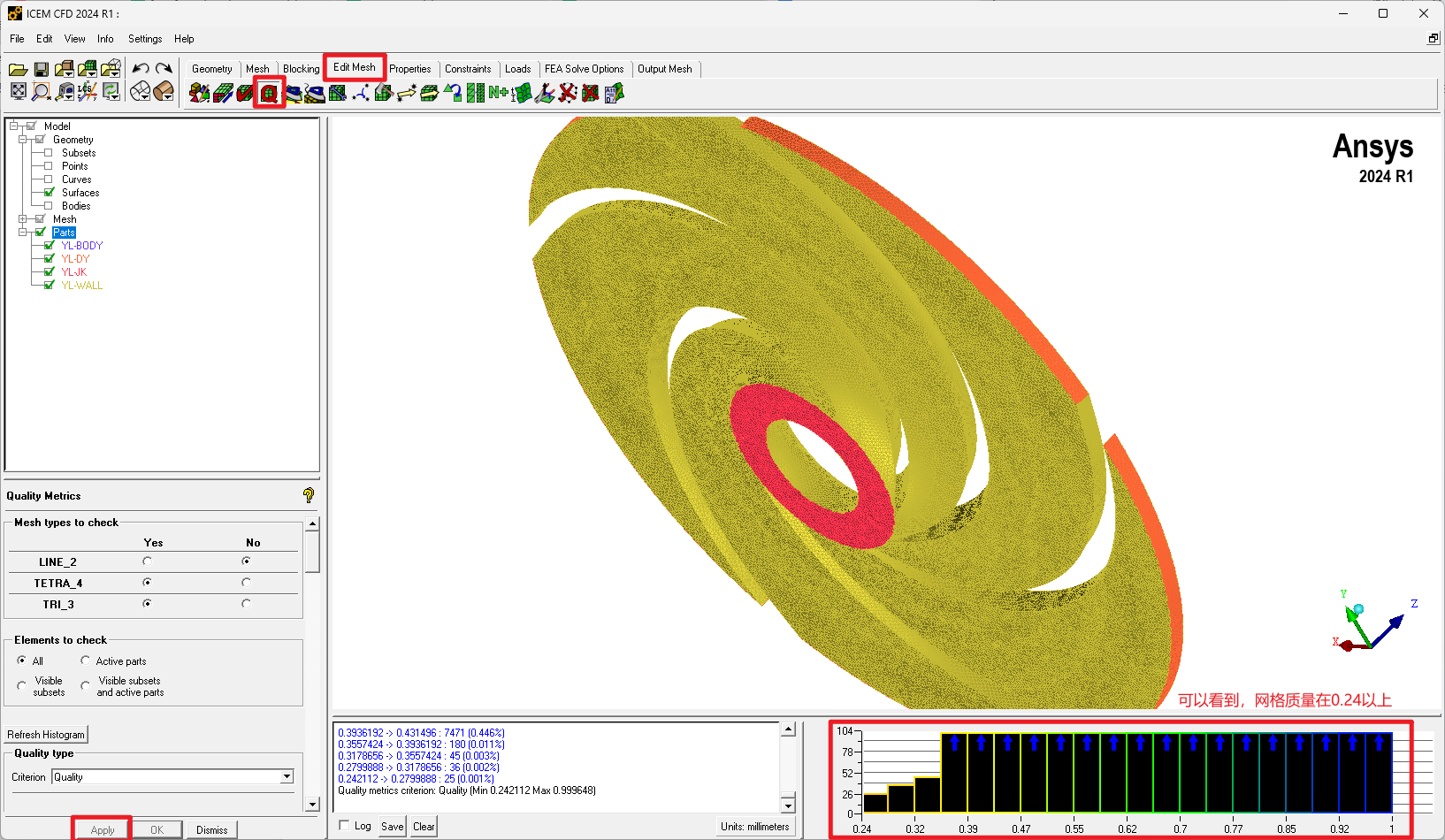
1.6.3 Check Mesh Quality

After mesh generation, the mesh quality must be checked. The following items should be emphasized:

• Whether the minimum orthogonal quality is too low;
• Whether the maximum skewness is too high;
• Whether negative-volume cells exist;
• Whether the mesh at the interfaces is continuous and complete;
• Whether the leading edge, trailing edge, guide-vane inlet, and other regions are too coarse.

If the mesh quality is poor, adjust the global mesh size, local mesh size, or geometry topology and then regenerate the mesh. For pump internal-flow simulations, mesh quality directly affects pressure pulsation, pump head, efficiency, and flow-field distribution results.

1.6.4 Rename the Mesh Body and Save the Mesh

In the Parts tree in the upper-left panel, select the generated mesh body and rename it, for example:

yl

Then save the mesh file:

File → Mesh → Save Mesh As

Enter a file name and save it. After completing the current component, close the file and continue meshing the other model components.

---

1.7 Merge and Export the Complete Mesh

After all components have been meshed, the individual meshes need to be merged into a complete model mesh.

1.7.1 Import and Merge Meshes

Open each mesh file in sequence by selecting:

File → Mesh → Open Mesh

During import, select Merge to merge multiple meshes into the same project.

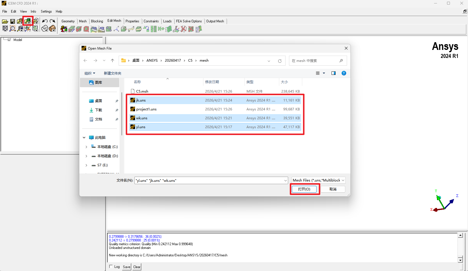
After merging, check whether the interfaces of different components have naming conflicts, missing boundaries, or position mismatches.

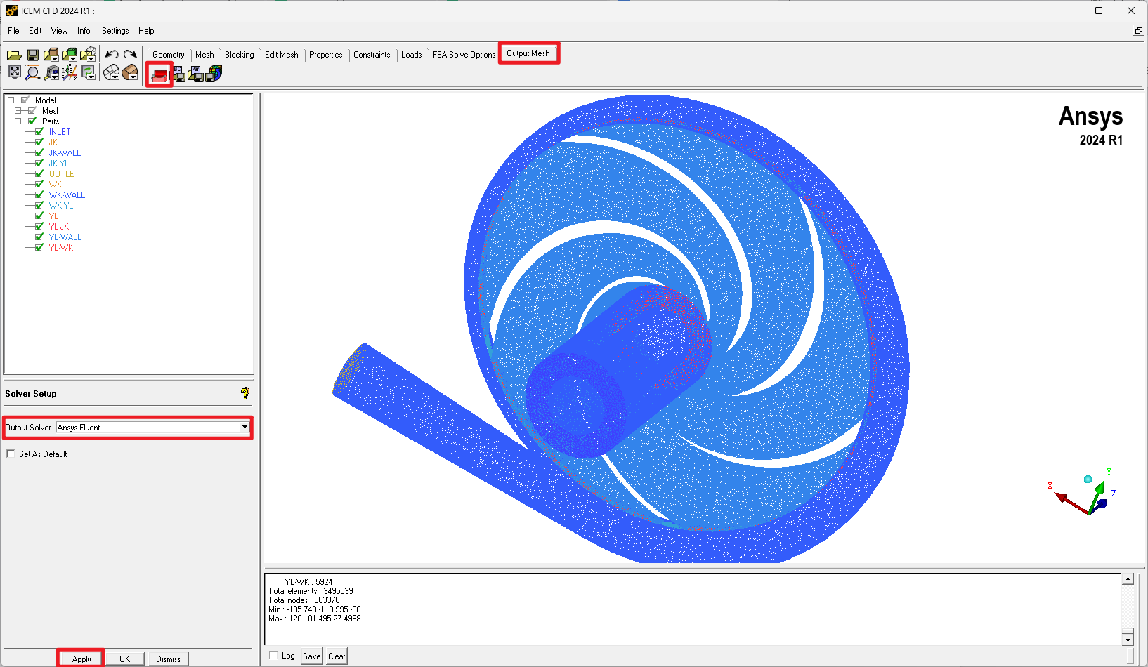
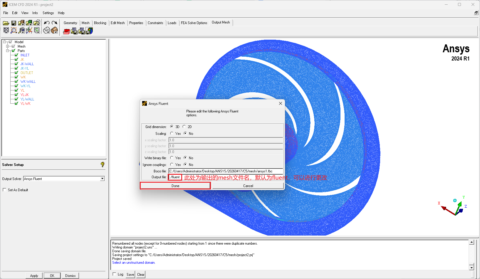
1.7.2 Select the Solver and Export the Mesh

To export a mesh file that can be read by Fluent, select:

Output Mesh → Select Solver → Apply

Then select:

Output Mesh → Write Input

Save the file according to the prompts, name the mesh, and finally click Done.

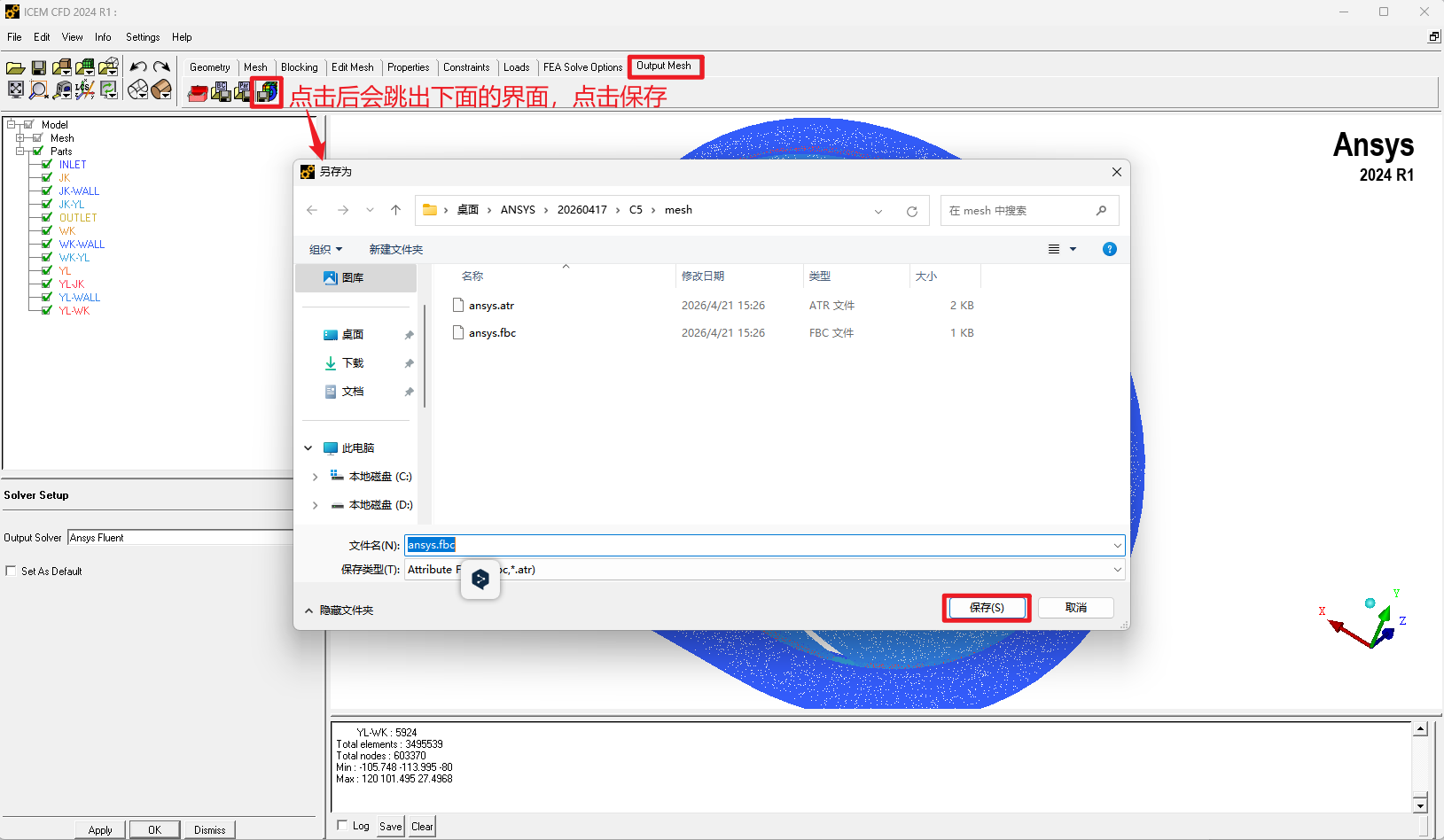
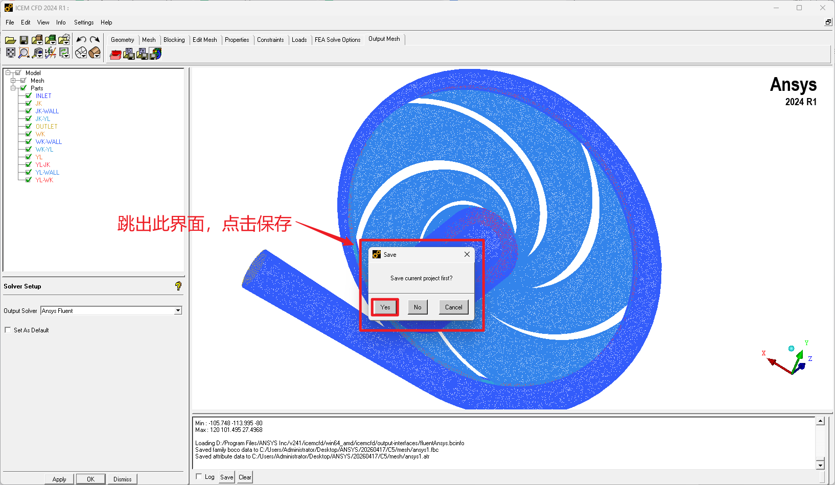
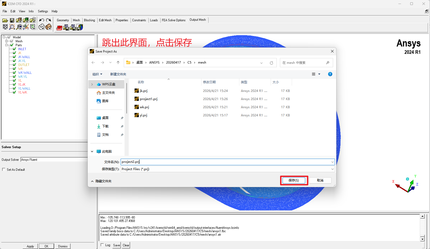
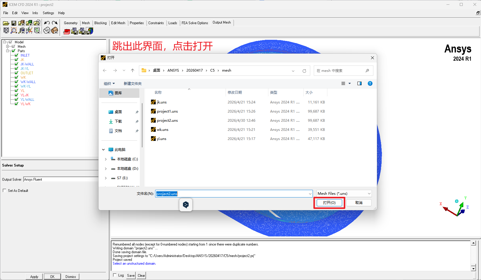
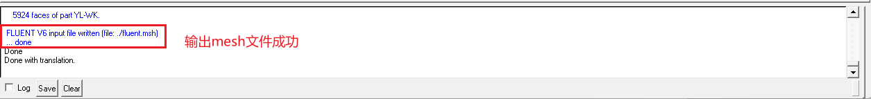
After export, find the generated mesh file in the working directory. It is usually a .msh file or another input file format that Fluent can read.

---

2. Steady-State Simulation in Fluent

2.1 Start Fluent and Import the Mesh

Start ANSYS Fluent and set the working directory to the same folder as the mesh file, or to another folder that is convenient for project management.

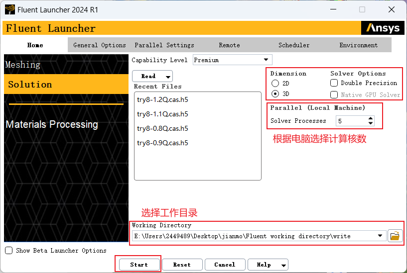
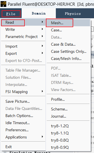
Import the mesh file exported from ICEM into Fluent and wait until the file is fully read.

After importing the mesh, it is recommended to run a mesh check first. Confirm that there are no negative-volume cells or severe mesh errors, and check whether the boundary names are consistent with those defined in ICEM.

---

2.2 Check Mesh Scale and Units

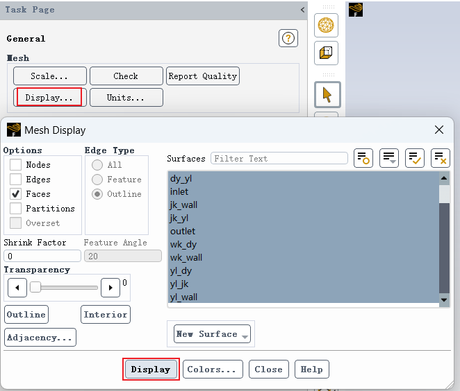
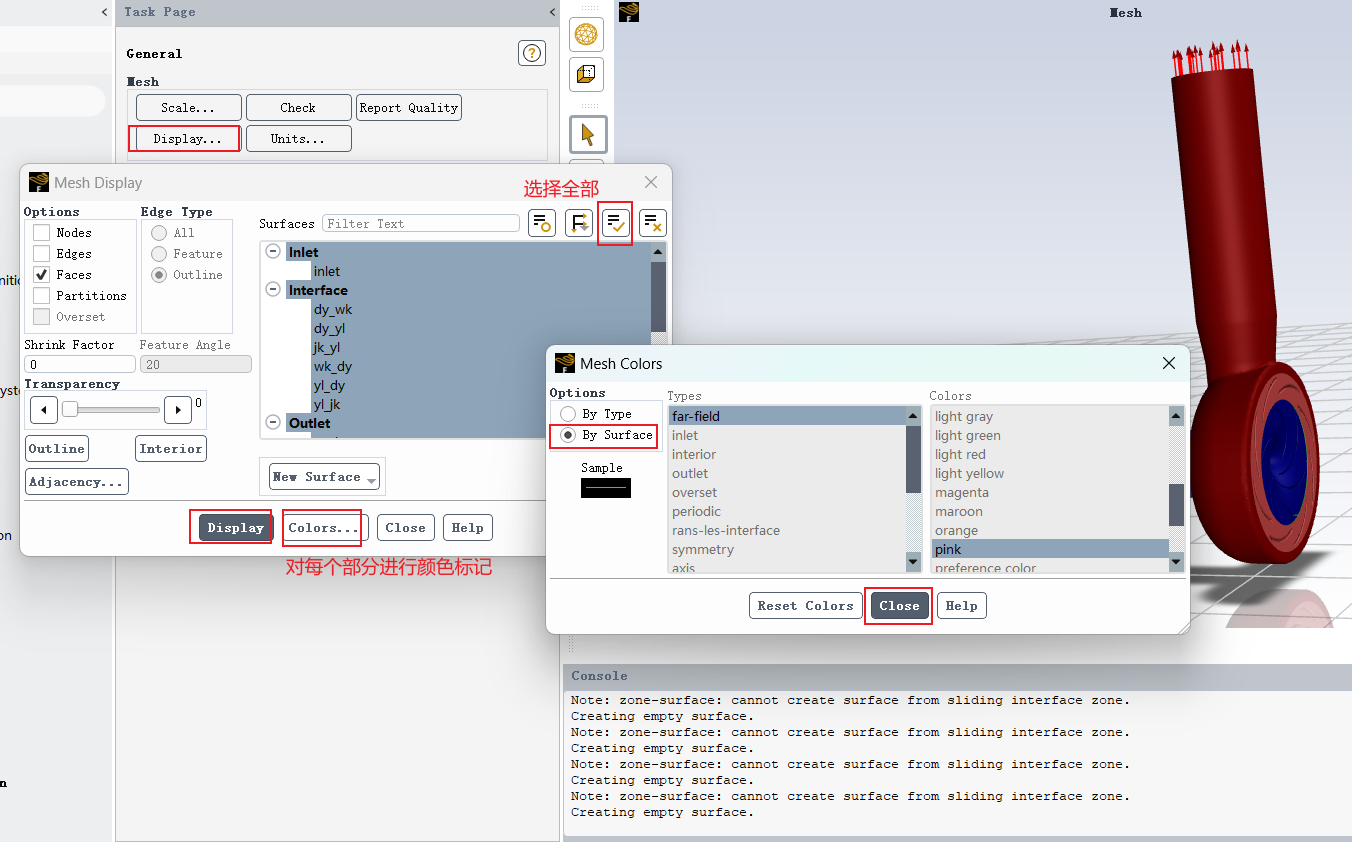
After importing the mesh, display the mesh and check the model dimensions. If millimeter was used in ICEM while Fluent uses meter as the default unit, the mesh scale must be checked or scaled correctly.

Common operations include:

Mesh → Check
Mesh → Scale
Display → Mesh

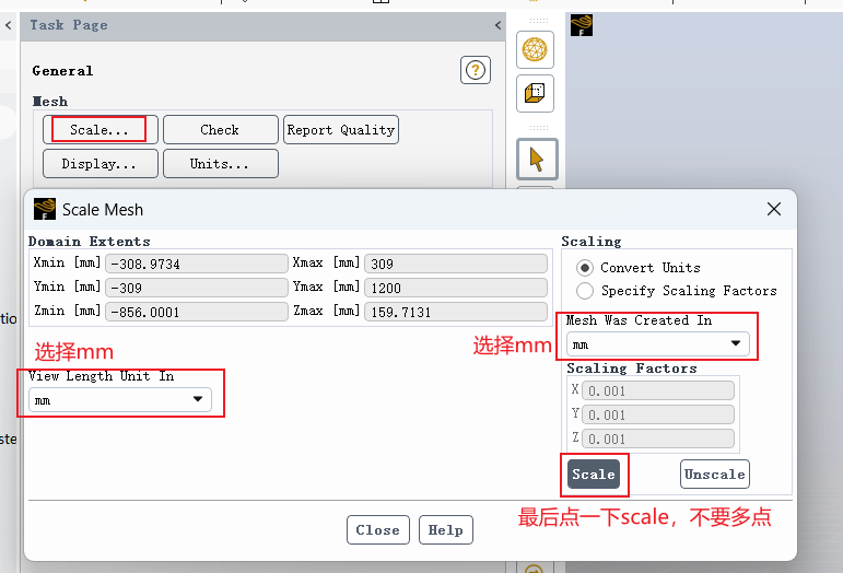
Note: Unit inconsistency is one of the most common problems in Fluent simulations. If the model size is enlarged or reduced by a factor of 1000, the velocity, flow rate, Reynolds number, pump head, and efficiency will all become incorrect.

---

2.3 Select the Physical Model and Fluid Medium

2.3.1 Select the Calculation Model

Select an appropriate turbulence model in Fluent according to the simulation requirements. This example is a steady-state simulation. Depending on the research purpose, models such as standard k-ε, RNG k-ε, realizable k-ε, or SST k-ω can be selected.

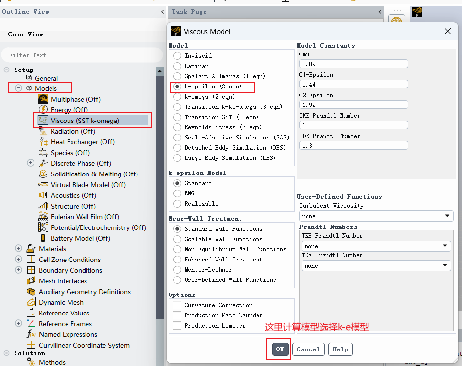
If near-wall separation, adverse pressure gradients, or complex internal flows in turbomachinery are of interest, the turbulence model should be selected together with the mesh y+ value and the research objective.

2.3.2 Set the Fluid Medium

Select the working fluid from the material library. In this example, water at room temperature is selected, so the density and viscosity are set according to the properties of water at normal temperature.

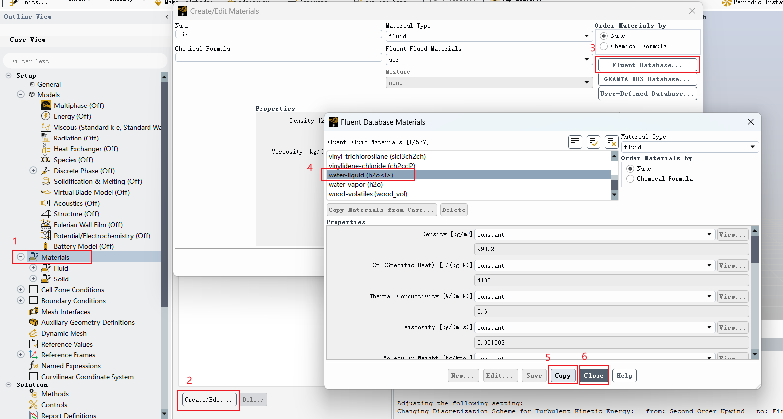
If the working medium is not water, the density, dynamic viscosity, and other physical properties should be modified according to the experimental or engineering conditions.

---

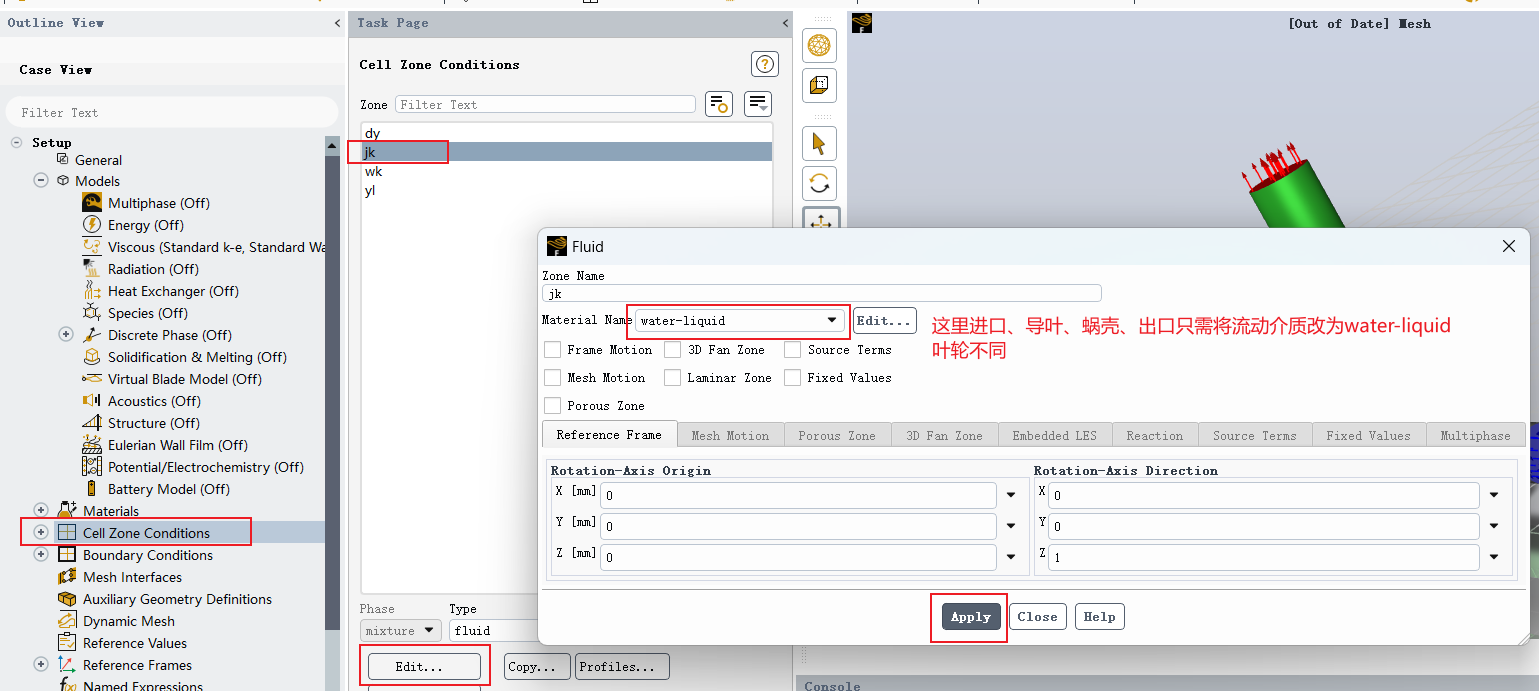
2.4 Set Cell Zone Conditions and the Rotating Domain

Set all fluid zones in Cell Zone Conditions. For pump models, the following zones usually need to be distinguished:

• Impeller rotating domain;
• Guide-vane or volute stationary domain;
• Inlet and outlet sections;
• Other auxiliary fluid regions.

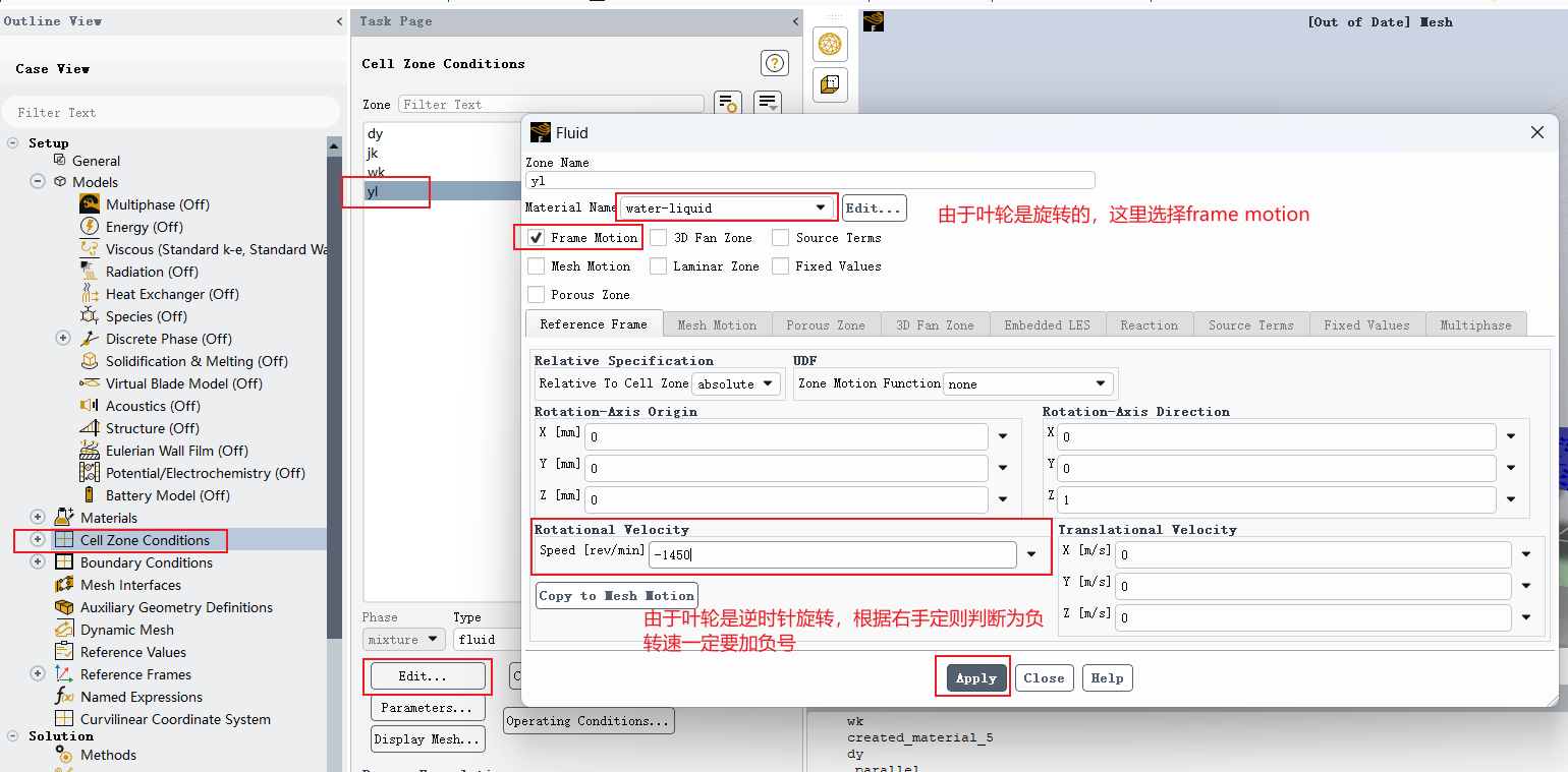
The sign of the impeller rotational speed must be determined according to the rotation-axis direction and the right-hand rule:

Point the thumb of your right hand along the positive direction of the rotation axis, for example the positive Z direction. The curled direction of the four fingers represents the positive rotation direction. If the actual impeller rotation direction is the same as the curled-finger direction, the rotational speed is positive. If it is opposite, the rotational speed is negative.

For example, if the impeller rotates around the Z axis, first determine the positive direction of the Z axis, and then determine the sign of the rotational speed according to the actual rotation direction.

---

2.5 Set Boundary Conditions

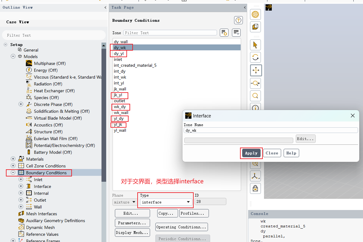
2.5.1 Interface Boundaries

First, confirm whether the interfaces defined in ICEM are correctly recognized in Fluent. Connection surfaces between the rotating domain and the stationary domain usually need to be set as interface boundaries, or used later to create mesh interfaces.

2.5.2 Inlet Boundary

The inlet can usually be set as a velocity inlet, mass-flow inlet, or pressure inlet. If the volume flow rate Q and inlet area A are known, the average inlet velocity can be set as:

$$v = \frac{Q}{A}$$

where:

• v is the average inlet velocity, in m/s;
• Q is the volume flow rate, in m³/s;
• A is the inlet cross-sectional area, in m².

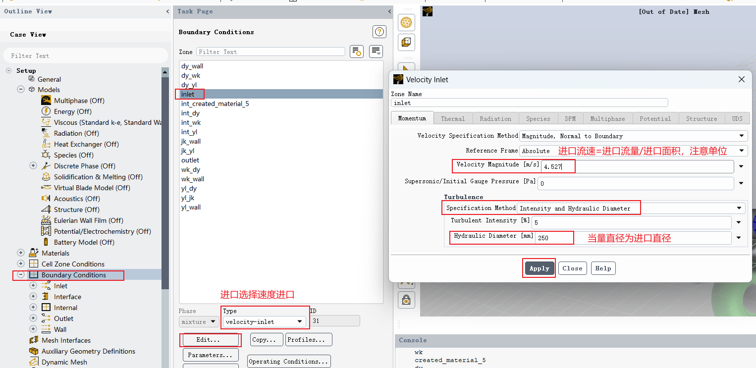
If the engineering flow rate is given in m³/h, it should first be converted into m³/s:

$$Q_{m^3/s} = \frac{Q_{m^3/h}}{3600}$$

2.5.3 Outlet Boundary

The outlet boundary can be set as a pressure outlet or another suitable boundary type according to the actual operating condition. When using a pressure outlet, pay attention to the backflow turbulence parameters and the outlet pressure reference value.

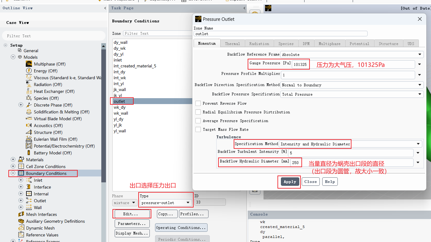
In the outlet boundary settings, the hydraulic diameter may need to be specified. For a non-circular cross-section, the hydraulic diameter is defined as:

$$D_e = \frac{4A}{P}$$

where:

• D_e is the hydraulic diameter, in m;
• A is the effective flow area, in m²;
• P is the wetted perimeter, in m. The wetted perimeter is the length of the boundary where the fluid contacts the solid wall on the effective cross-section.

For a fully filled annular cross-section, if the outer diameter is D_o and the inner diameter is D_i, the hydraulic diameter is:

$$D_e = D_o - D_i$$

2.5.4 Impeller Wall Boundary

The impeller wall should be defined according to the rotating-domain setup. If the impeller is located in a rotating reference frame, the wall is usually set as stationary relative to the adjacent rotating zone or moving with the rotating domain, depending on the modeling approach.

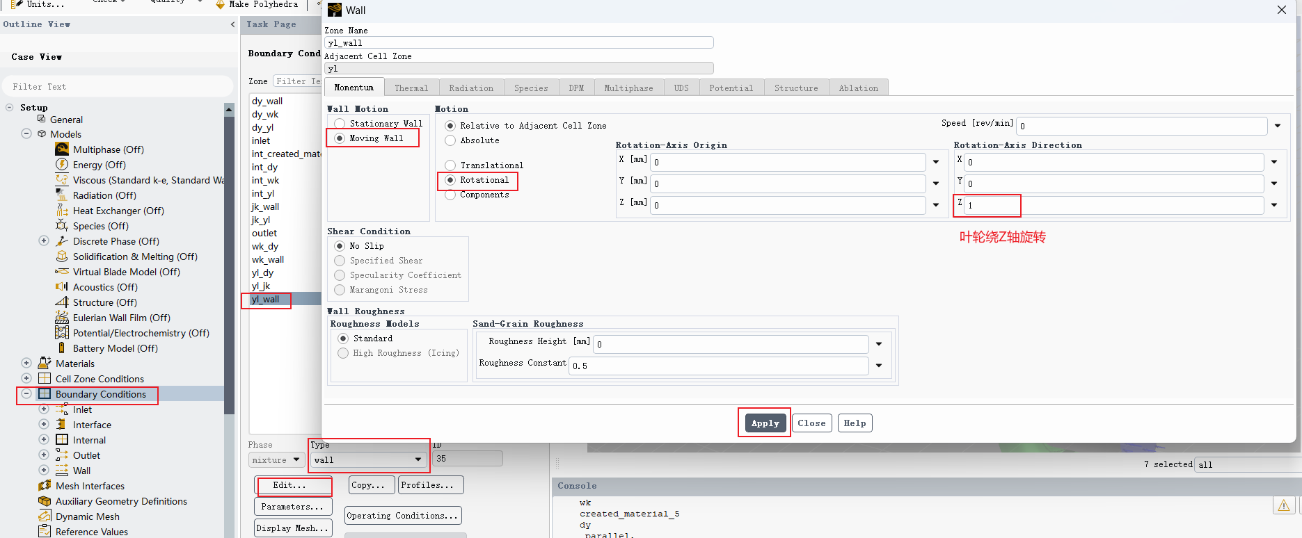
Note: The rotating domain, wall motion, and coordinate-system settings must be consistent. If these settings are incorrect, the relative velocity and pressure distribution on the blade surface may become obviously unreasonable.

---

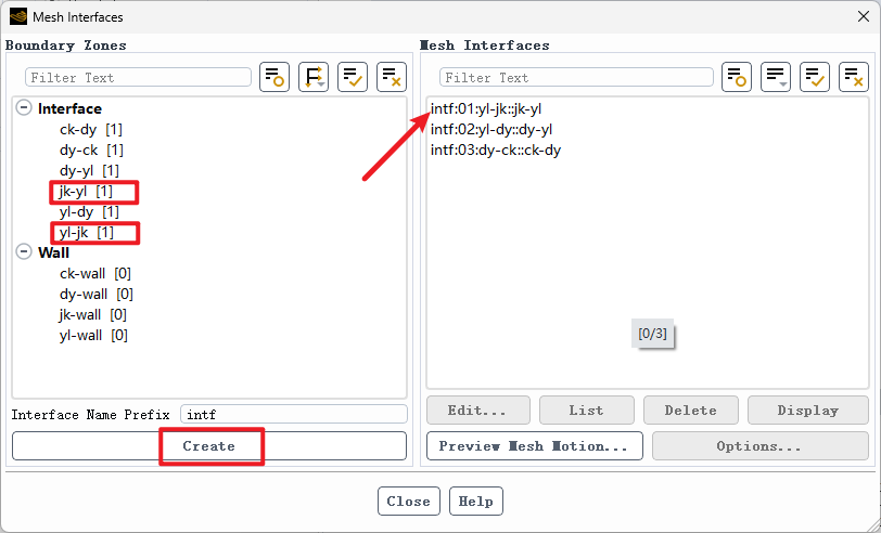
2.6 Create Mesh Interfaces

In Fluent, corresponding interface surfaces must be paired so that flow-field information can be transferred between the rotating and stationary domains.

Method 1: Automatically Select Interfaces

If the boundary names are standardized and the interface surfaces match well, the corresponding interfaces can be selected directly and saved.

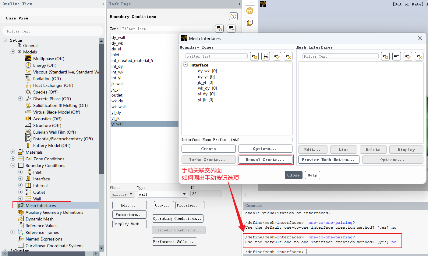
Method 2: Manually Create a Mesh Interface

If automatic recognition fails or there are many interface names, the mesh interface can be created manually.

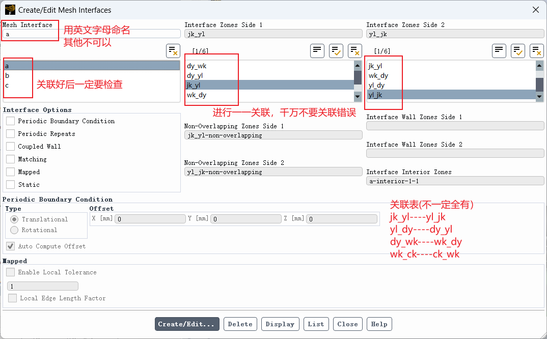
After creation, check the number of interfaces, the paired relationships, and the interface directions.

---

2.7 Solution Methods, Convergence Criteria, and Initialization

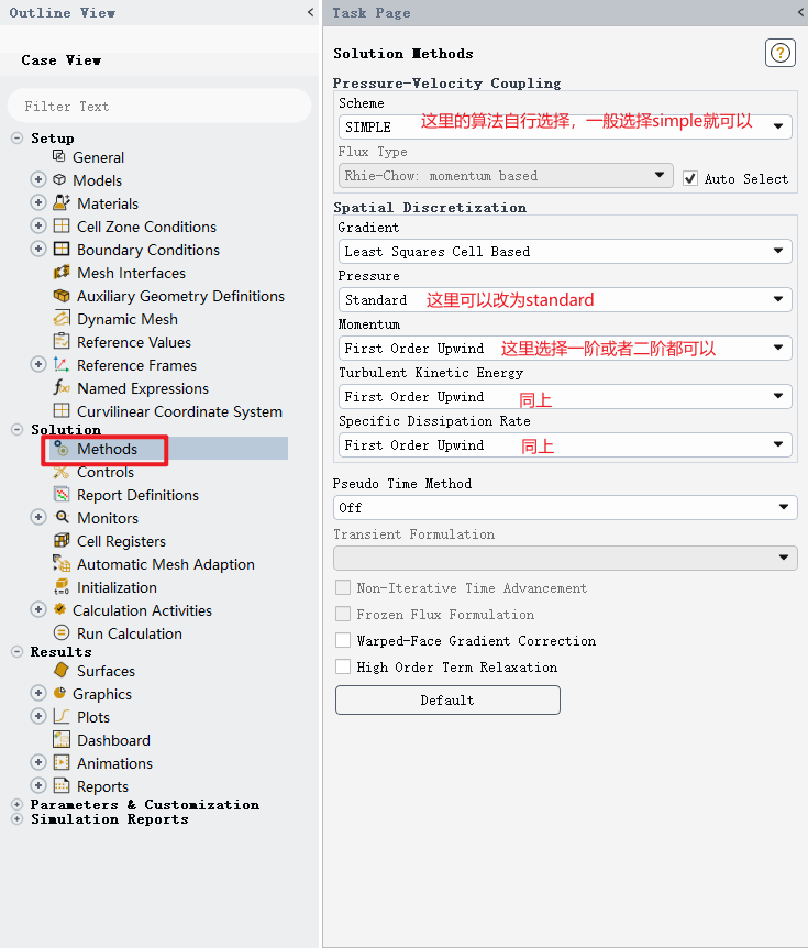
2.7.1 Set the Solution Method

In Solution Methods, choose the pressure-velocity coupling method, discretization schemes, and gradient calculation method. For steady-state pump internal-flow simulations, SIMPLE or Coupled methods are commonly used. The final choice depends on numerical stability and convergence speed.

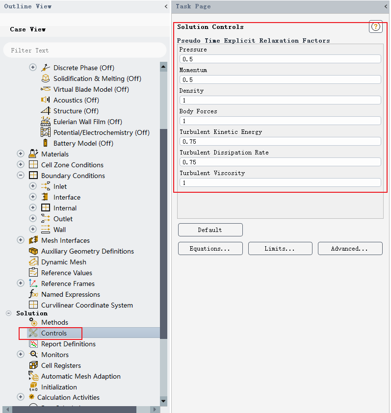
2.7.2 Set Solution Controls

In Solution Controls, relaxation factors can be adjusted. For the initial calculation, the default settings can be used. If divergence occurs or the residuals oscillate strongly, the relaxation factors for pressure, momentum, or turbulence variables can be reduced appropriately.

2.7.3 Set Convergence Criteria

Set the convergence criteria in Residual Monitors. In this example, the residual criterion can be set to 1e-9, and the maximum number of iterations can be set to, for example, 3000.

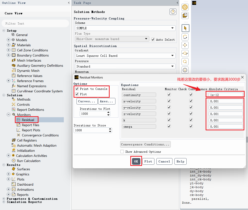
However, convergence should not be judged only by the number of iterations. The following items should also be checked:

• Whether all equation residuals decrease and become stable;
• Whether the inlet and outlet mass flow rates are balanced;
• Whether monitored quantities such as pump head, efficiency, and torque are stable;
• Whether periodic oscillation or local divergence still exists.

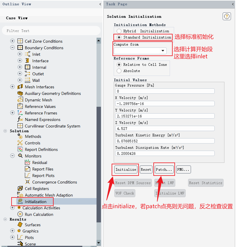
2.7.4 Initialization

After completing the settings, initialize the flow field. Standard initialization or hybrid initialization can be used.

---

2.8 Run Iterations and Save Data

After initialization, start the iterative solution.

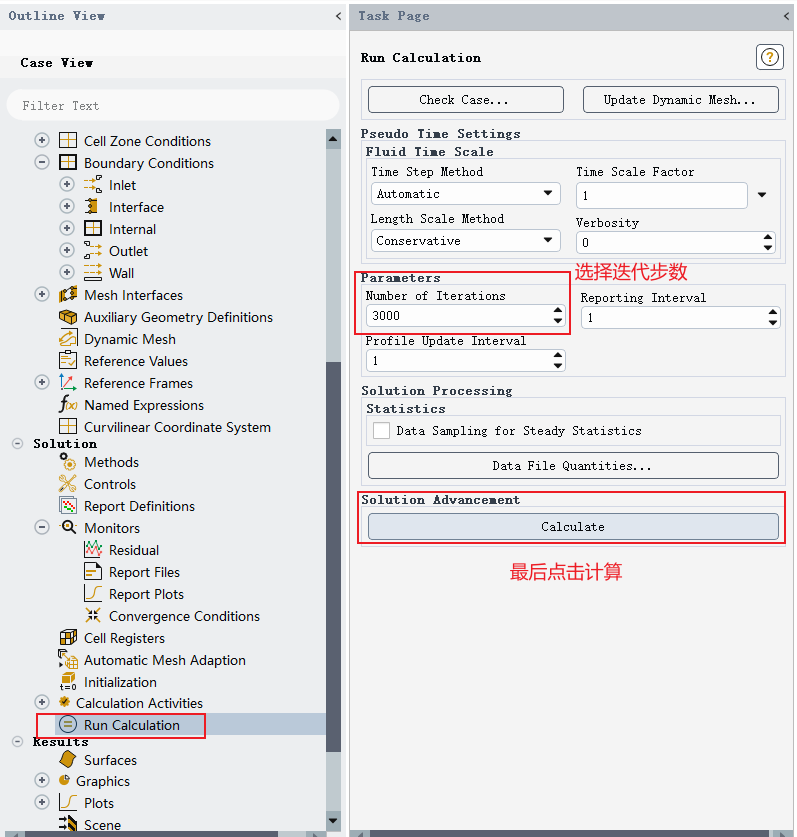
After the calculation is completed, save the results in time:

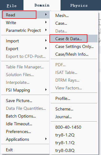
File → Write → Case & Data

It is recommended to save both .cas and .dat files, so that the simulation can be continued later or used for post-processing.

---

3. Post-Processing in Fluent

This section uses the built-in post-processing functions in Fluent to analyze the simulation results.

3.1 Import the Computed Data

Open Fluent and import the completed case and data files.

---

3.2 Calculate Pump Head

The pump head can be calculated from the total pressure difference between the outlet and the inlet. The general formula is:

$$H = \frac{p_{out} - p_{in}}{\rho g} + \Delta z$$

where:

• H is the pump head, in m;
• p_out is the outlet pressure, in Pa;
• p_in is the inlet pressure, in Pa;
• ρ is the fluid density, in kg/m³;
• g is the gravitational acceleration, usually taken as 9.81 m/s²;
• Δz is the elevation difference between the outlet and inlet pressure-measurement sections, in m.

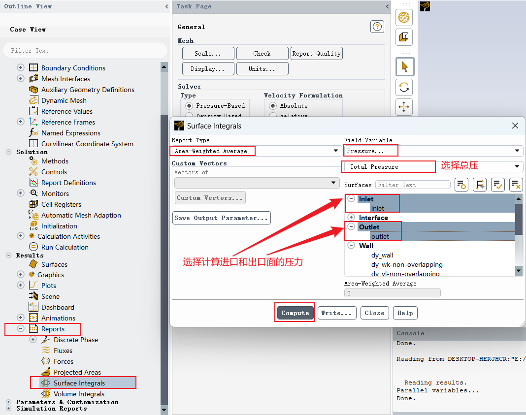
An example of the inlet and outlet pressure calculation result is shown below.

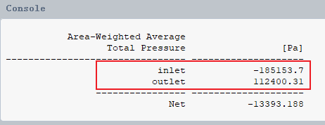
If, in the example, the outlet pressure is 112400.31 Pa, the inlet pressure is -185153.7 Pa, the density is 1000 kg/m³, and the elevation difference is temporarily ignored, the pump head is:

$$H = \frac{112400.31 - (-185153.7)}{1000 \times 9.81}$$

If the elevation difference between the inlet and outlet sections cannot be ignored, the Δz term should be included in the calculation.

---

3.3 Calculate Pump Efficiency

Pump efficiency is obtained from the ratio of hydraulic power to shaft input power:

$$\eta = \frac{P_e}{P}$$

where the hydraulic power is:

$$P_e = \rho g Q H$$

The shaft input power can be calculated from torque and rotational speed:

$$P = T \omega = T \frac{2\pi n}{60} = T \frac{\pi n}{30}$$

where:

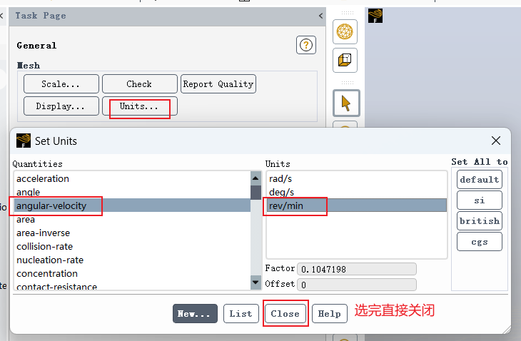
• η is the pump efficiency;
• P_e is the hydraulic power of the pump, in W;
• P is the shaft input power, in W;
• T is the torque, in N·m;
• ω is the angular velocity, in rad/s;
• n is the rotational speed, in r/min;
• Q is the flow rate, in m³/s;
• H is the pump head, in m.

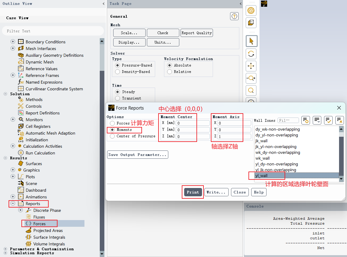
The moment center should be selected according to the model coordinate system and rotation axis. This must be determined based on the specific model. The sign of the torque calculated by Fluent represents direction. For efficiency calculation, the absolute value of the torque is usually used.

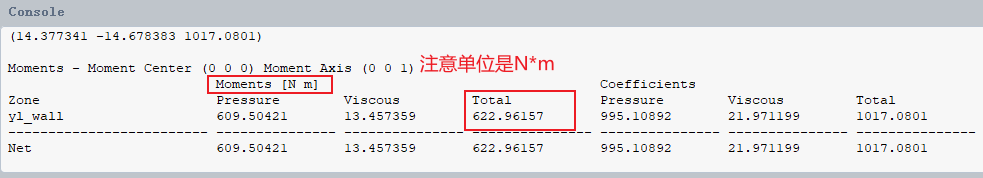
The example calculation is as follows:

Torque: T = 622.96157 N·m
Rotational speed: n = 1450 r/min
Flow rate: Q = 800 / 3600 m³/s

The shaft input power is:

$$P = 622.96157 \times 1450 \times \frac{\pi}{30}$$

The hydraulic power is:

$$P_e = 1000 \times 9.81 \times \frac{800}{3600} \times H$$

The pump efficiency is:

$$\eta = \frac{P_e}{P}$$

---

3.4 Plot Flow-Field Contours

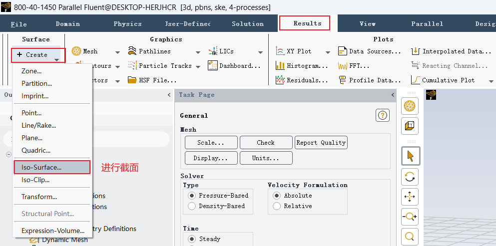
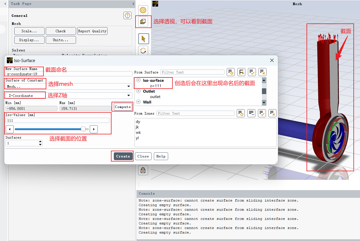
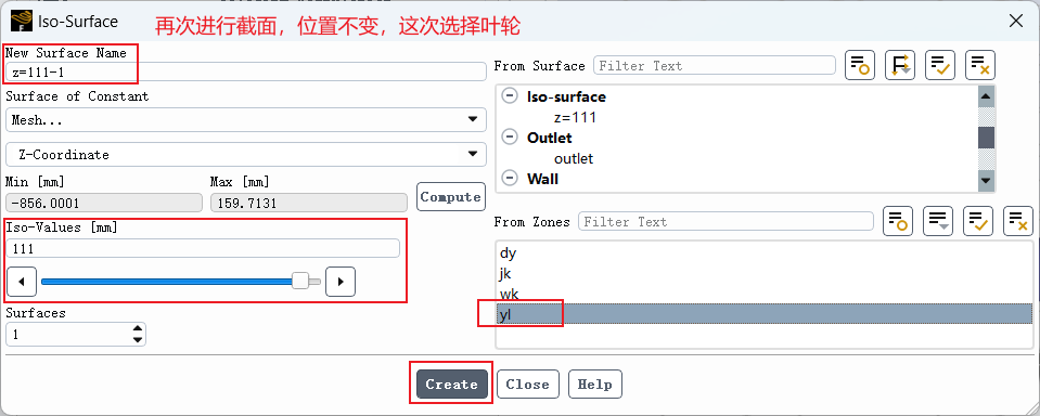
3.4.1 Create Section Planes

Before plotting pressure, velocity, or other contours, create section planes for displaying the results. The section location can be selected according to the analysis purpose, such as the impeller mid-plane, guide-vane mid-plane, inlet section, or outlet section.

3.4.2 Pressure Contour

Select the pressure variable and display the contour on the created section plane. When plotting pressure contours, pay attention to the unit, legend range, and color-band distribution. An overly wide legend range may hide local pressure variations.

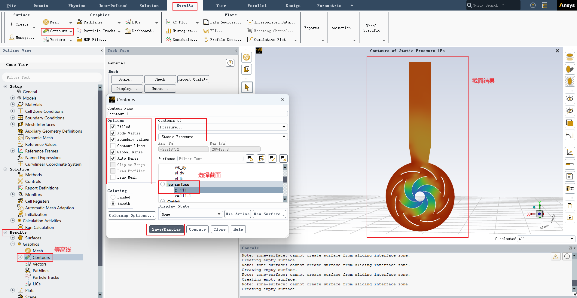
After the settings are completed, export the result image.

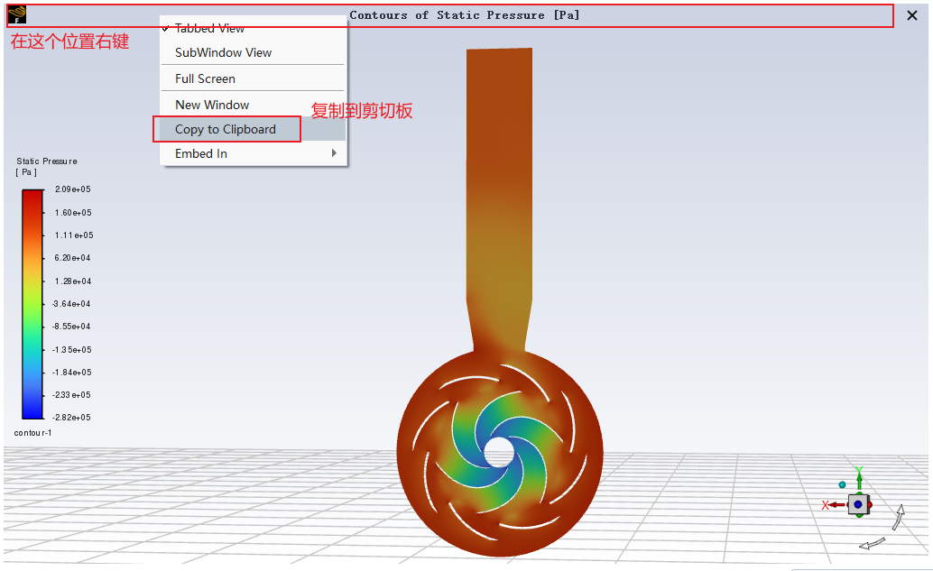
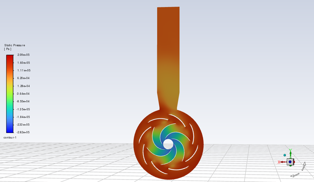
An example pressure contour result is shown below.

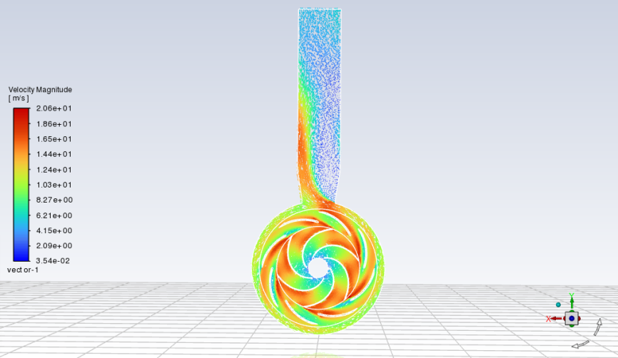
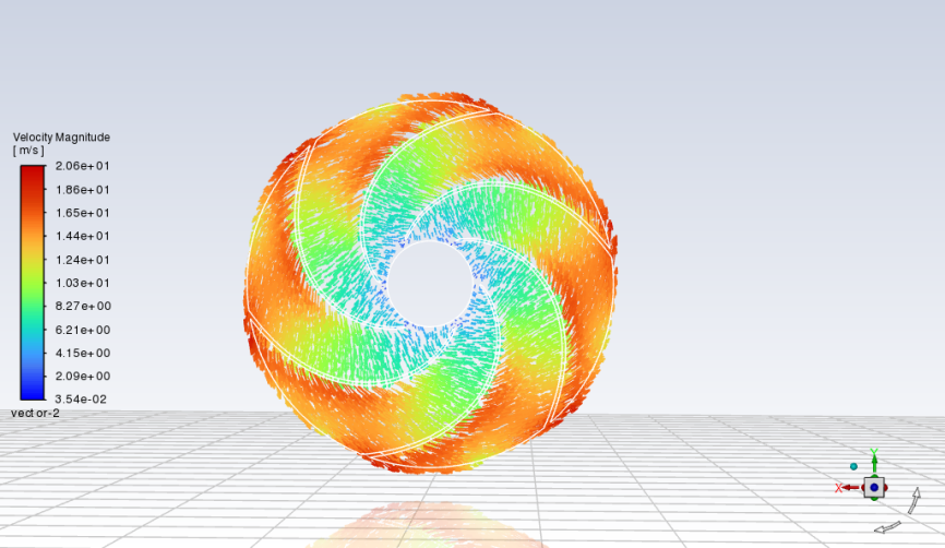
3.4.3 Absolute Velocity Contour

The absolute velocity contour is used to observe the velocity distribution in the stationary reference frame. It is suitable for analyzing overall flow acceleration, diffusion, and separation regions.

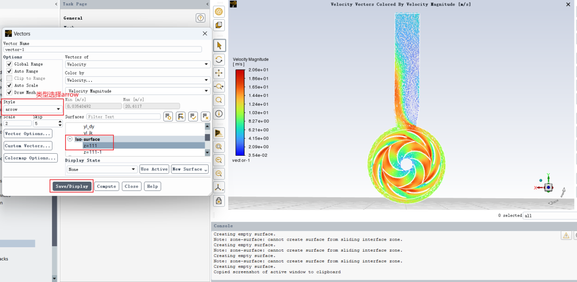
An example absolute velocity contour result is shown below.

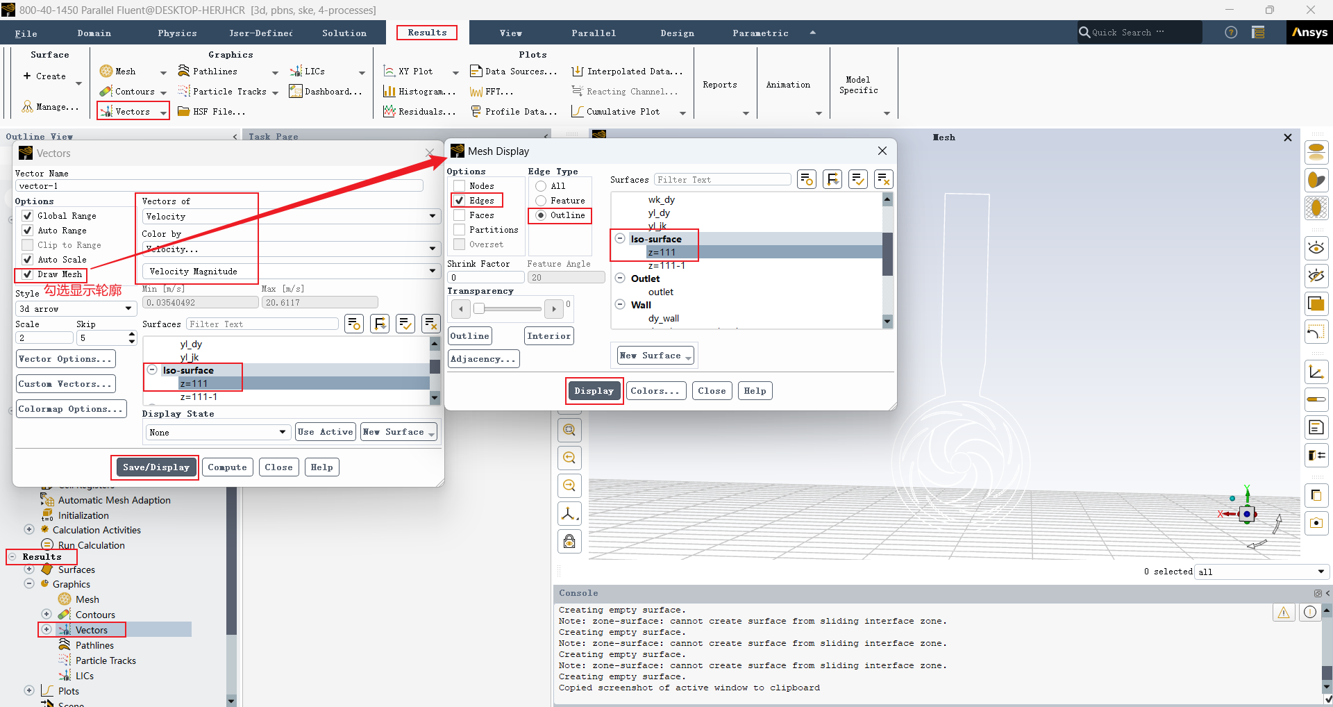
3.4.4 Relative Velocity Contour in the Impeller

For the impeller relative velocity contour, the correct relative reference region must be selected. For flow inside the impeller, the reference region should be changed to the impeller rotating domain. Otherwise, the obtained velocity field may not represent the result in the impeller relative coordinate system.

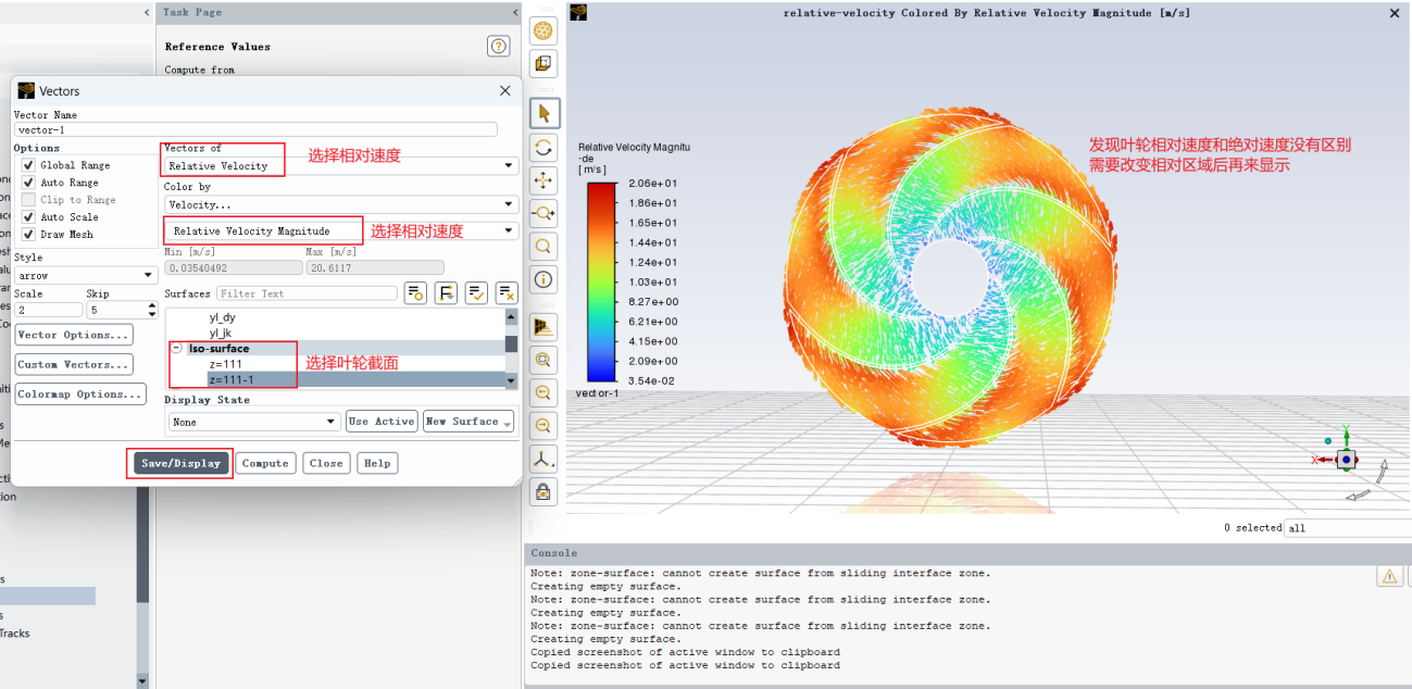
Change the relative reference region.

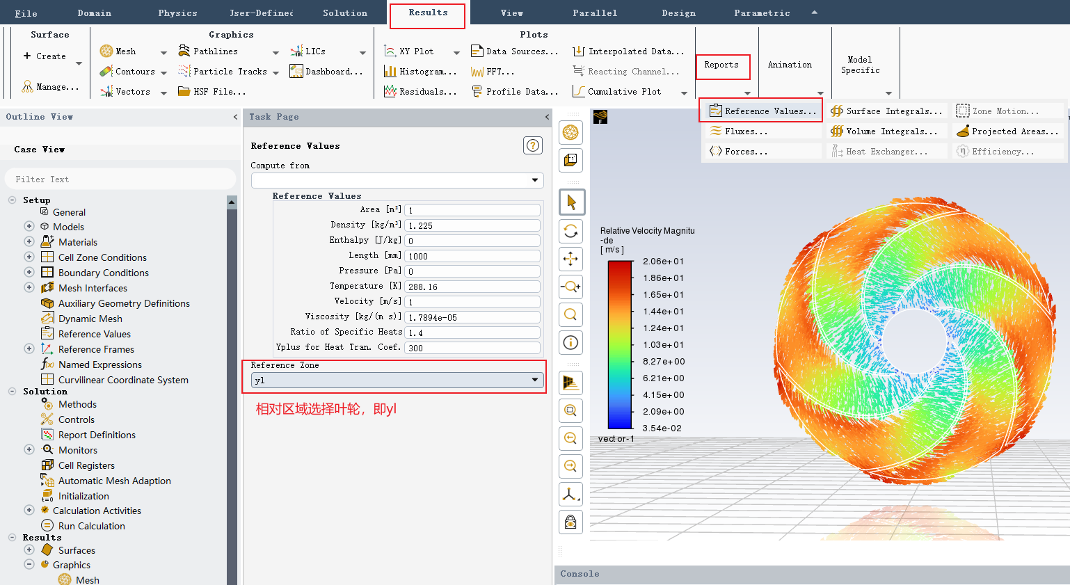
The adjusted relative velocity contour is shown below.

---

4. Post-Processing in CFD-Post

In addition to the built-in post-processing functions in Fluent, CFD-Post can also be used for visualizing section planes, contours, vectors, streamlines, and other results.

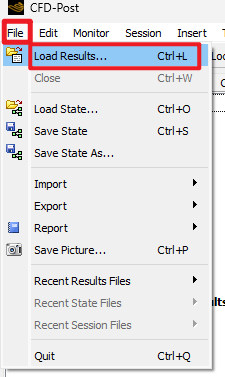
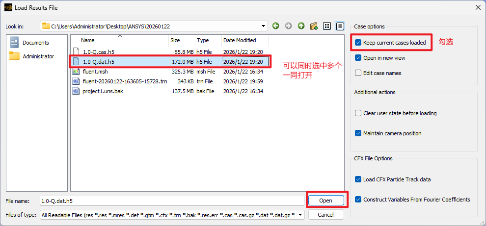
4.1 Import the Data File

Start CFD-Post and import the .dat file obtained from Fluent. If necessary, import the corresponding case file as well.

---

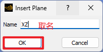
4.2 Create a Section Plane

Create a plane section in CFD-Post to display pressure, velocity, and other variable distributions.

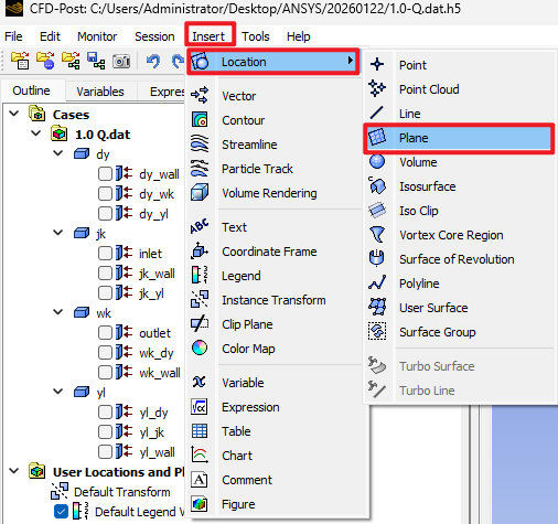
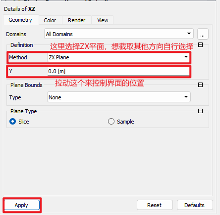
When creating a section plane, confirm whether the section direction, coordinate position, and display range meet the analysis requirements.

---

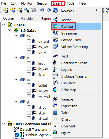
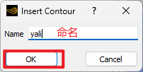
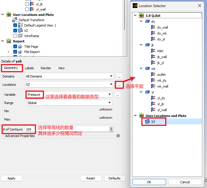
4.3 Create Contour Plots

Create a Contour and specify the displayed variable, display location, and color range. For example, static pressure, total pressure, absolute velocity, or relative velocity can be selected.

Tips for view adjustment:

• Hold Ctrl and scroll the middle mouse wheel to rotate the view;
• Click the corresponding coordinate axis to switch to a front view perpendicular to that axis;
• Adjust the model orientation and zoom ratio to make the contour clearer.

---

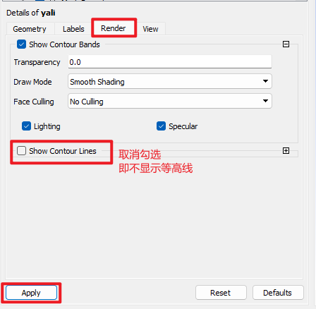
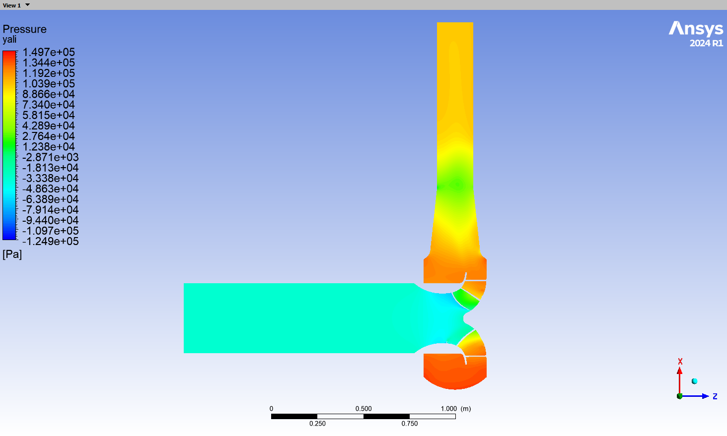
4.4 Adjust the Legend and Display Style

To make the result image more visually clear and quantitatively accurate, adjust the legend range, number of color bands, font size, and legend position. For contour plots used in papers or reports, it is recommended to keep the legend range consistent within the same comparison group. Otherwise, the colors in different figures cannot be compared directly.

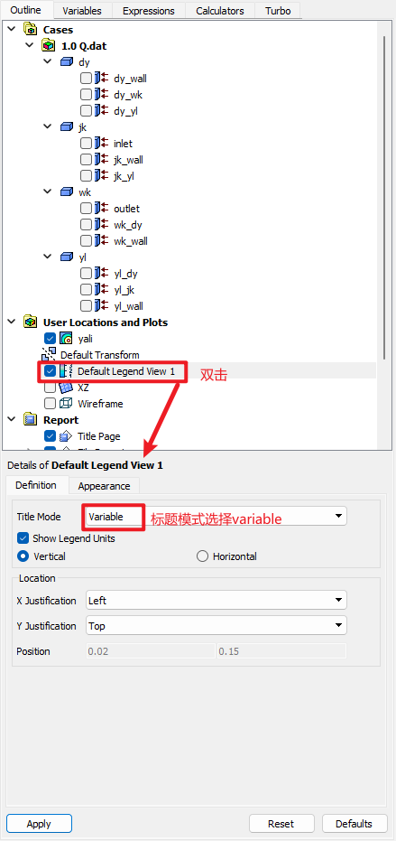
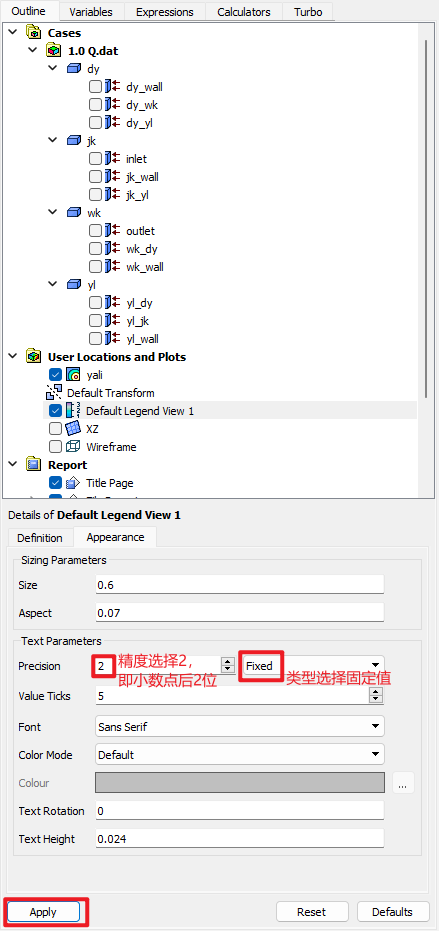
An adjusted pressure contour example is shown below.

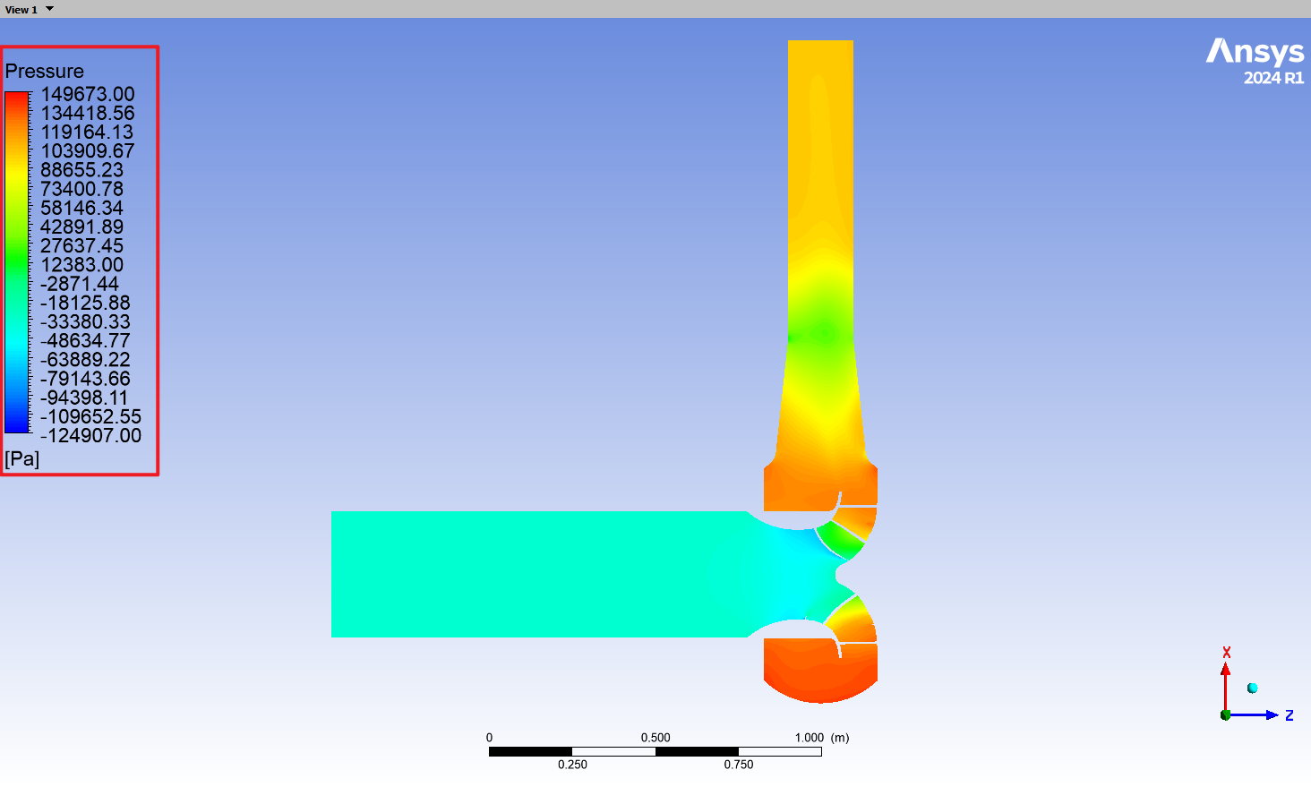
The method for plotting velocity contours is similar to that for pressure contours. The only difference is that the displayed variable should be changed to the corresponding velocity variable.

---

5. Common Notes and Recommendations

1. Use an English-only working path when possible. ICEM, Fluent, and CFD-Post may not always handle Chinese characters or special symbols in file paths reliably, especially when reading mesh files or writing result files.

2. Keep geometry units consistent. The unit selected when importing the model into ICEM must be consistent with the mesh scale in Fluent. After importing the mesh into Fluent, the model dimensions must be checked.

3. Use standardized boundary names. The inlet, outlet, wall, interface, rotating-domain, and stationary-domain boundary names should be clearly distinguished. Recommended names include inlet, outlet, yl-wall, yl-jk, and jk-yl. The use of underscores in all the attached images in this article is incorrect; the correct form should be a hyphen "-".

4. Check interfaces in pairs. Incorrect interface settings between the rotating and stationary domains may cause discontinuous flow fields, abnormal residuals, or unreasonable simulation results.

5. Confirm the rotation direction using the right-hand rule. An incorrect sign for the impeller rotational speed will directly lead to wrong directions in the pump head, velocity field, and pressure field.

6. Do not judge convergence only by residuals. In addition to residuals, pump head, torque, efficiency, and mass-flow conservation should also be monitored. If these quantities still fluctuate significantly, the calculation should not be considered fully converged even if the residuals have decreased.

7. Keep post-processing legends consistent. When comparing a group of pressure or velocity contours, use the same legend range and color-band settings so that the results are comparable.

8. Save results frequently. After completing each important step, save the project, mesh, case, and data files to avoid data loss caused by unexpected software shutdowns.