1. Basic Idea of POD

Proper Orthogonal Decomposition (POD) is a widely used method for data reduction and modal decomposition. It extracts the most energetic and representative structures from complex datasets such as flow fields, pressure fields, or experimental measurements.

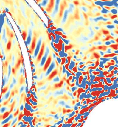
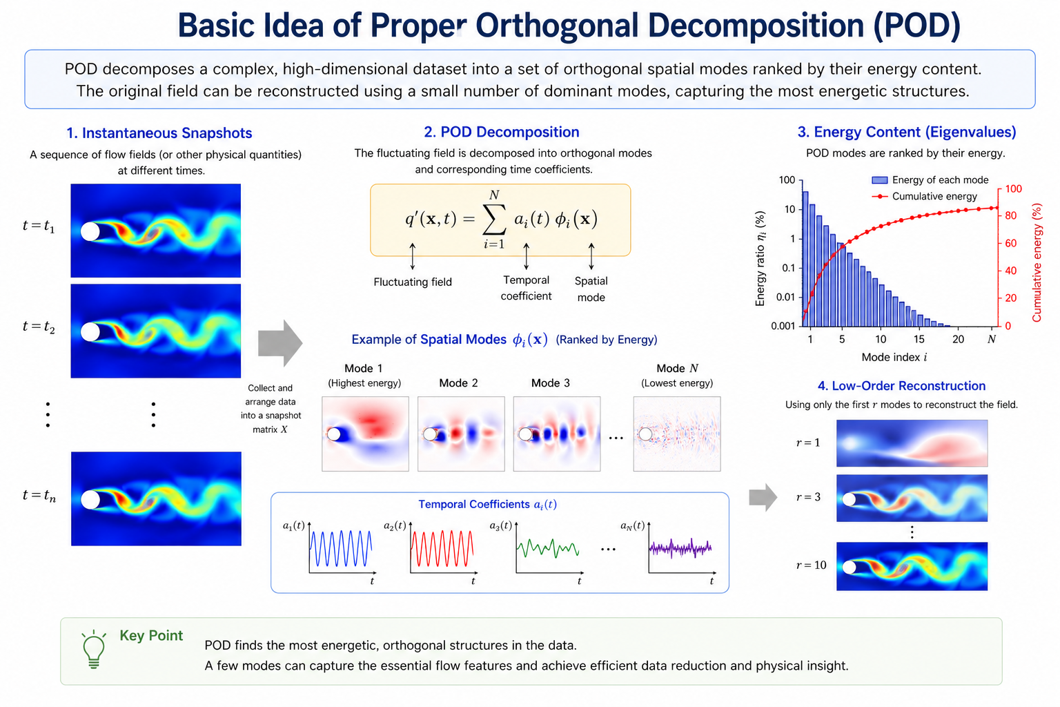
The core idea of POD is to represent a complex system using a limited number of orthogonal modes that capture the maximum possible energy. For flow field analysis, POD decomposes a transient field into a set of spatial modes and corresponding temporal coefficients, revealing dominant coherent structures in the flow.

Compared with directly analyzing a large number of instantaneous snapshots, POD significantly simplifies the problem by identifying a few dominant modes, making it easier to interpret flow structures, energy distribution, and unsteady behavior.

2. Mathematical Formulation of POD

Let the instantaneous field be denoted as $q(\mathbf{x}, t)$ , where $\mathbf{x}$ is the spatial coordinate and $t$ is time. POD aims to express it as:

q(\mathbf{x}, t) = \overline{q}(\mathbf{x}) + \sum_{i=1}^{N} a_i(t)\phi_i(\mathbf{x})

where:

$\overline{q}(\mathbf{x})$ is the mean field
$\phi_i(\mathbf{x})$ is the $i$ -th spatial POD mode
$a_i(t)$ is the corresponding temporal coefficient
$N$ is the number of modes

In practice, the fluctuating component is first obtained:

q'(\mathbf{x}, t) = q(\mathbf{x}, t) - \overline{q}(\mathbf{x})

Then POD is applied to the fluctuating field:

q'(\mathbf{x}, t) = \sum_{i=1}^{N} a_i(t)\phi_i(\mathbf{x})

3. Physical Meaning of POD Modes

The spatial modes $\phi_i(\mathbf{x})$ represent dominant flow structures. The first mode usually contains the highest energy and corresponds to the most significant coherent structure. Higher-order modes contain progressively less energy and often represent smaller-scale or more complex structures.

The temporal coefficients $a_i(t)$ describe how each spatial mode evolves over time.

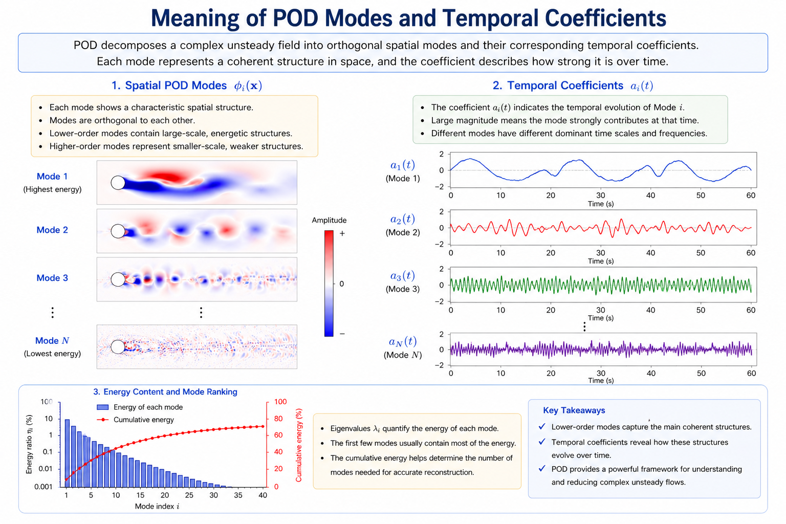
Each POD mode is associated with an eigenvalue $\lambda_i$ , which represents its energy contribution. The energy ratio of the $i$ -th mode is:

\eta_i = \frac{\lambda_i}{\sum_{j=1}^{N} \lambda_j}

The cumulative energy of the first $r$ modes is:

\eta_{\mathrm{cum}}(r) = \frac{\sum_{i=1}^{r} \lambda_i}{\sum_{j=1}^{N} \lambda_j}

If a few modes capture most of the energy, the system exhibits low-dimensional characteristics.

4. Basic Procedure of POD

The general procedure of POD analysis is as follows:

Collect transient data (velocity, pressure, vorticity, etc.)
Convert each snapshot into a column vector
Construct the snapshot matrix
Perform decomposition to obtain modes, coefficients, and energies
Analyze dominant structures based on energy contribution

For $m$ spatial points and $n$ snapshots, the snapshot matrix is:

\mathbf{X} = \begin{bmatrix} | & | & & | \\ \mathbf{x}_1 & \mathbf{x}_2 & \cdots & \mathbf{x}_n \\ | & | & & | \end{bmatrix} \in \mathbb{R}^{m \times n}

SVD-Based POD (SVD-POD)

5. Basic Idea of SVD-POD

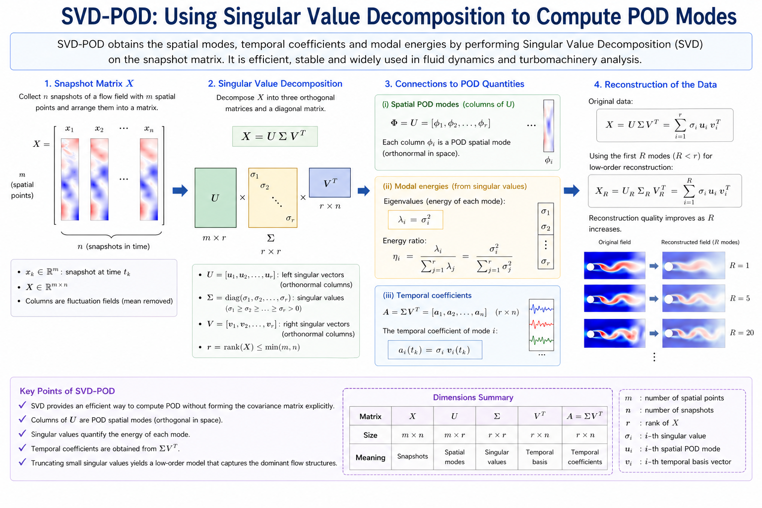
SVD-POD is a numerical implementation of POD using Singular Value Decomposition (SVD). Instead of explicitly forming the covariance matrix, SVD directly decomposes the snapshot matrix, making it computationally efficient and stable.

For the snapshot matrix $\mathbf{X}$ , SVD is given by:

\mathbf{X} = \mathbf{U}\mathbf{\Sigma}\mathbf{V}^T

where:

$\mathbf{U}$ contains left singular vectors (spatial modes)
$\mathbf{\Sigma}$ is a diagonal matrix of singular values
$\mathbf{V}$ contains right singular vectors (time information)

6. Derivation of SVD-POD

Given the snapshot matrix:

\mathbf{X} = \begin{bmatrix} \mathbf{x}_1 & \mathbf{x}_2 & \cdots & \mathbf{x}_n \end{bmatrix}

Perform SVD:

\mathbf{X} = \mathbf{U}\mathbf{\Sigma}\mathbf{V}^T

where:

\mathbf{\Sigma} = \mathrm{diag}(\sigma_1, \sigma_2, \cdots, \sigma_r)

with:

\sigma_1 \geq \sigma_2 \geq \cdots \geq \sigma_r > 0

The POD modes are given by:

\mathbf{\Phi} = \mathbf{U}

The energy associated with each mode is proportional to the square of the singular values:

\lambda_i = \sigma_i^2

Thus, the energy ratio is:

\eta_i = \frac{\sigma_i^2}{\sum_{j=1}^{r} \sigma_j^2}

and the cumulative energy is:

\eta_{\mathrm{cum}}(r) = \frac{\sum_{i=1}^{r} \sigma_i^2}{\sum_{j=1}^{N} \sigma_j^2}

7. Temporal Coefficients

In SVD-POD, the temporal coefficients can be obtained as:

\mathbf{A} = \mathbf{\Sigma}\mathbf{V}^T

Thus, the snapshot matrix can be reconstructed as:

\mathbf{X} = \mathbf{U}\mathbf{A}

or in summation form:

\mathbf{X} = \sum_{i=1}^{r} \sigma_i \mathbf{u}_i \mathbf{v}_i^T

For the $i$ -th mode, the temporal coefficient at time $t_k$ is:

a_i(t_k) = \sigma_i v_i(t_k)

8. Low-Order Reconstruction

One key application of POD is reduced-order reconstruction. By retaining only the first $r$ dominant modes:

\mathbf{X}_r = \sum_{i=1}^{r} \sigma_i \mathbf{u}_i \mathbf{v}_i^T

or:

\mathbf{X}_r = \mathbf{U}_r \mathbf{\Sigma}_r \mathbf{V}_r^T

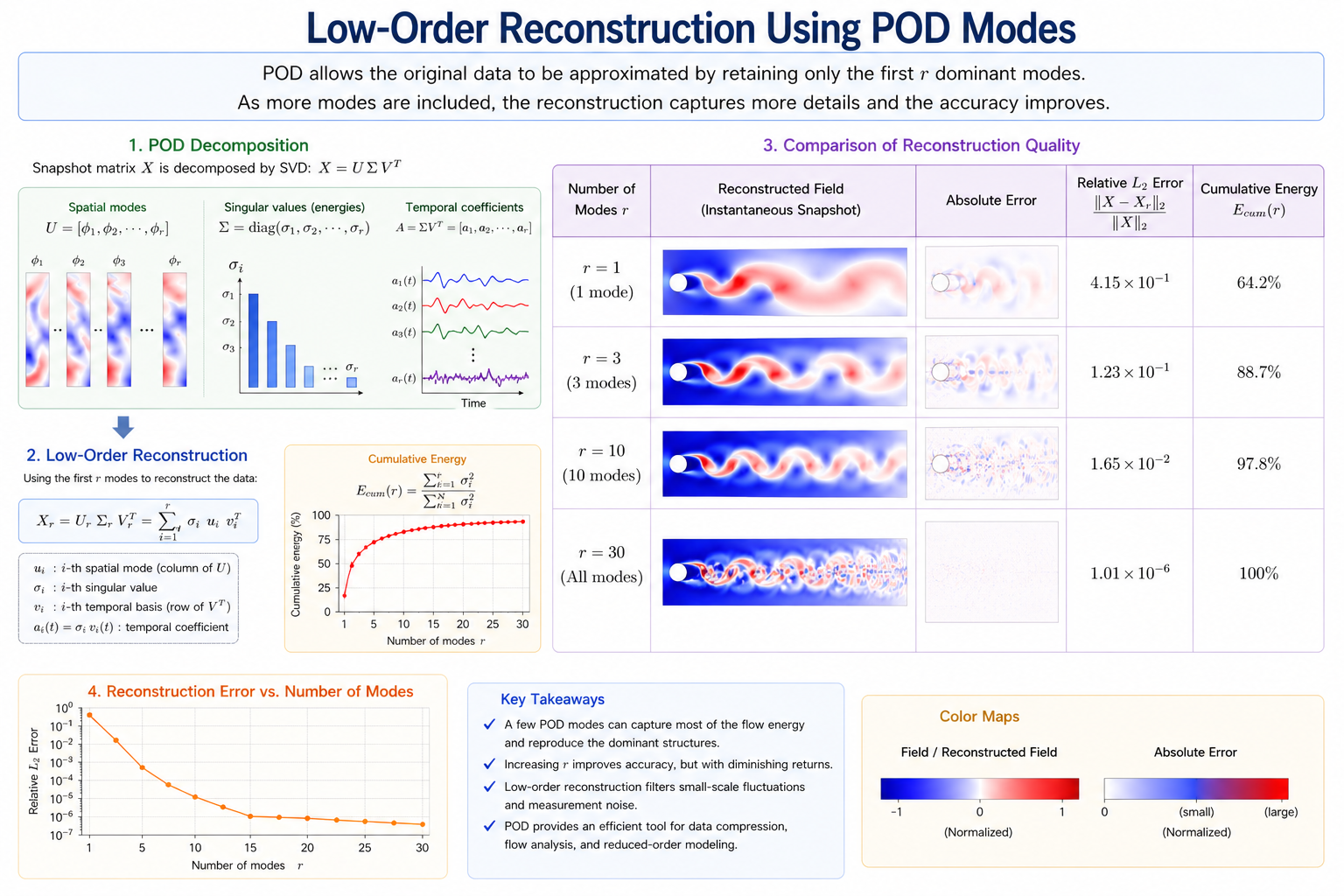
A small number of modes can capture the main structures while filtering out noise. Increasing $r$ improves reconstruction accuracy.

9. Relationship Between POD and SVD

POD is a theoretical framework for optimal energy-based decomposition, while SVD is a numerical tool used to compute POD modes.

In practice:

\text{POD provides the concept, SVD provides the computation}

10. Applications in Flow Analysis

POD is widely used in fluid mechanics and turbomachinery:

Extraction of dominant coherent structures
Analysis of energy distribution
Identification of large-scale vortices
Data dimensionality reduction
Low-order reconstruction
Separation of dominant structures and disturbances

For example, in pump flow analysis, low-order modes often correspond to major vortices, recirculation zones, or large-scale unsteady structures, while higher-order modes may represent small-scale turbulence or noise.

11. Advantages and Limitations

Advantages:

Optimal energy representation
Strong data compression capability
Clear identification of dominant structures

Limitations:

Modes are ranked by energy, not frequency
Multiple physical phenomena may be mixed in one mode

Therefore, additional analysis (e.g., FFT, HHT, or wavelet transform) is often needed to interpret modal frequency characteristics.

12. Summary

Proper Orthogonal Decomposition (POD) is an energy-based modal decomposition method that extracts dominant structures from complex datasets:

q'(\mathbf{x}, t) = \sum_{i=1}^{N} a_i(t)\phi_i(\mathbf{x})

SVD-POD implements POD using singular value decomposition:

\mathbf{X} = \mathbf{U}\mathbf{\Sigma}\mathbf{V}^T

Here, $\mathbf{U}$ represents spatial modes, $\mathbf{\Sigma}$ represents modal energy, and $\mathbf{V}$ describes temporal evolution.

POD is highly effective for extracting coherent structures, analyzing energy distribution, and performing reduced-order modeling, especially in unsteady flow analysis.