At the beginning.
The last tutorial update was almost five months ago. The previous one was about high-dimensional FFT, but the findings from pressure-pulsation analysis are ultimately quite limited. Since things have been less busy recently, I decided to post an update on coupling entropy-production theory with LES. Hopefully, it will be helpful for your research.
What is the entropy production theory?
For a pump, because of fluid viscosity and Reynolds stresses, part of the mechanical energy delivered by the motor is irreversibly converted into internal energy, leading to significant energy losses. Using the entropy-production approach makes it easy to visualize how unfavorable flow phenomena cause these losses and to evaluate the overall energy dissipation inside the pump.
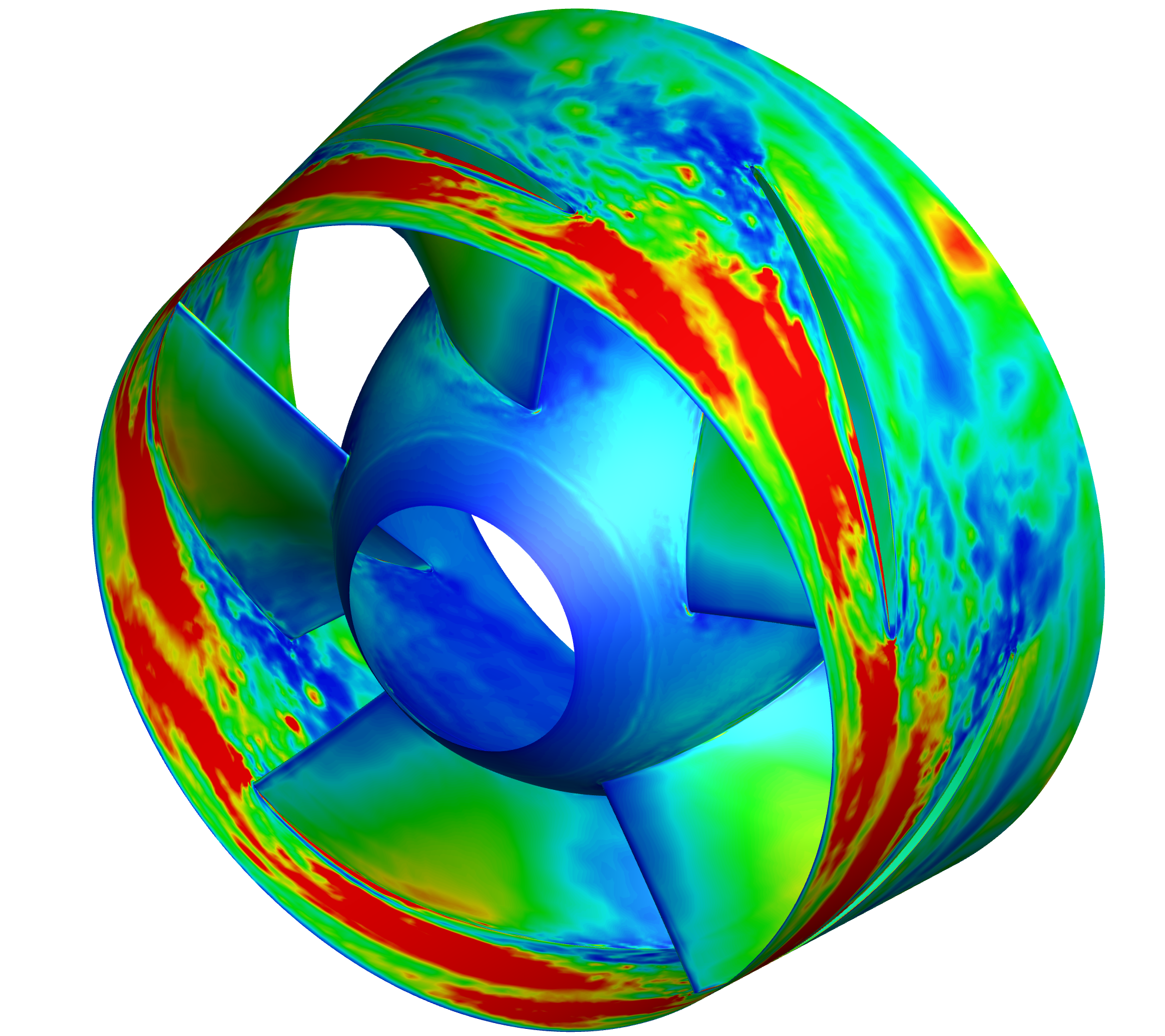
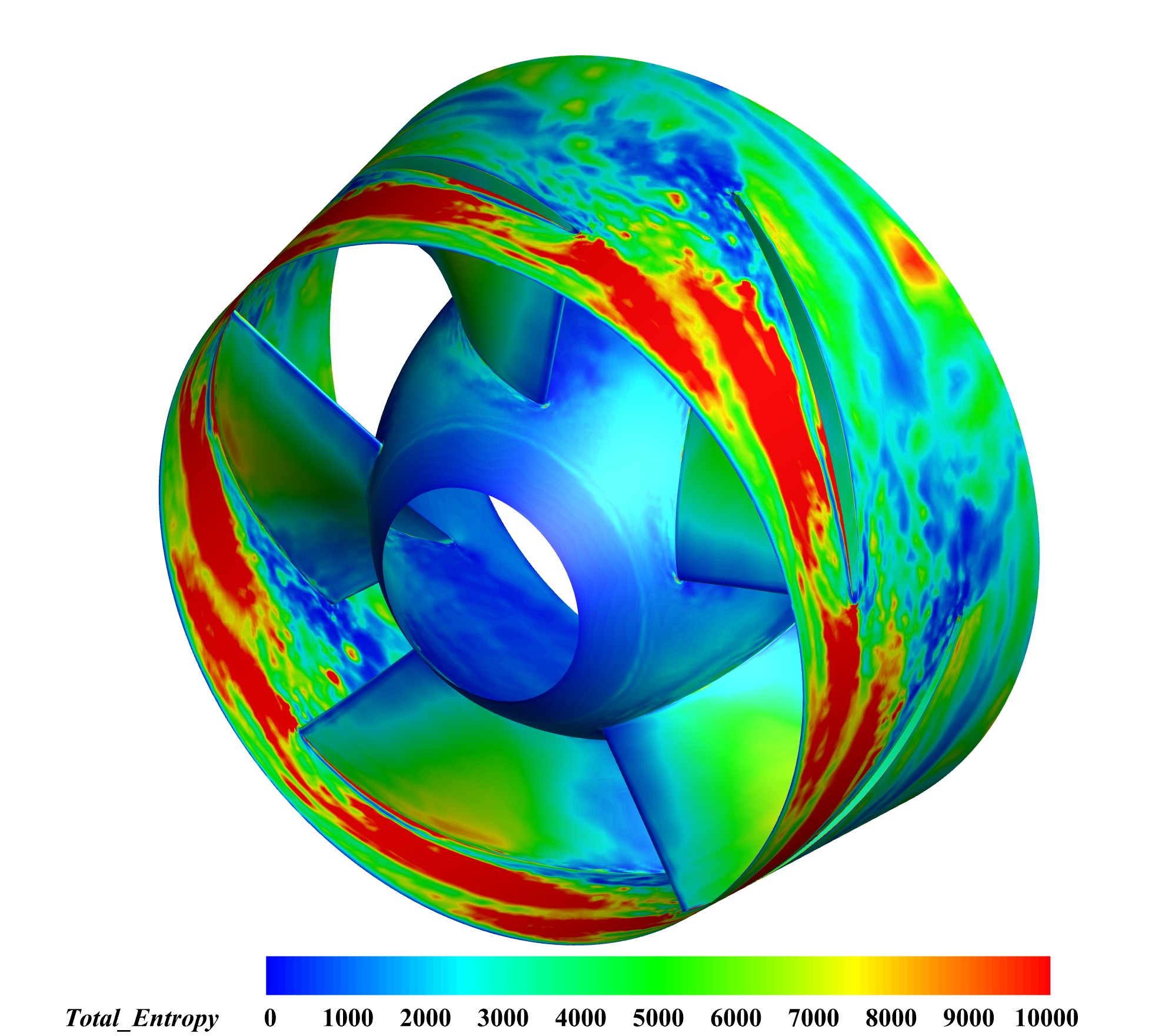
The figure below shows the entropy-production loss on the blade surface of an axial-flow pump impeller.
It’s worth noting that most previous studies calculated entropy production based on RANS results, while very few have done so using LES data. This tutorial will skip the background discussion of entropy-production theory and focus only on the essential formulas and how to couple entropy-production analysis with LES using ANSYS Fluent, MATLAB, and Tecplot.
According to the entropy-production theory proposed by Fabian Kock, entropy generation consists of two parts: viscous dissipation and heat transfer entropy production. In practical engineering applications, the temperature variation caused by the rotation of pump blades has a negligible effect on the fluid, so temperature change is often ignored for simplification. Therefore, in this study, only viscous-dissipation-related entropy production is considered. The viscous entropy production can be divided into direct viscous dissipation and turbulent viscous dissipation, expressed as follows:
Since the RANS model is based on time-averaged equations, the fluctuating terms in the governing equations cannot be directly computed. A common approach is to solve the internal flow field using the SST model, and then estimate the entropy production caused by turbulent viscous dissipation through the relationship among the turbulent dissipation rate , the turbulent kinetic energy , and the local temperature . The entropy production of turbulent viscous dissipation can be written as:
and
Here, is the specific dissipation rate, is the fluid density, is the turbulent kinetic energy, is the dissipation rate of turbulent kinetic energy, and is an empirical coefficient in the transport equation of turbulent kinetic energy, typically taken as .
However, this approach may introduce certain computational errors. Because it relies on simplified or indirect formulations to estimate entropy production, it may overlook local flow variations or the small-scale structures induced by turbulent fluctuations. As a result, noticeable deviations may appear between numerical predictions and the actual physical behavior. Ideally, the most accurate method should be based on a fully resolved representation of the turbulent flow field.
In general, taking a directional partial derivative of data is not easy to implement. However, Tecplot provides built-in functions for computing partial derivatives, which makes this task much more convenient. How to use these functions in Tecplot will be explained later in this tutorial.
Step 1. Preparatory work: setting up monitoring surfaces and preparing the data.
The procedure for setting up monitoring surfaces is the same as in the high-dimensional FFT tutorial, so it will not be repeated here. For more details, you can click here for more details.
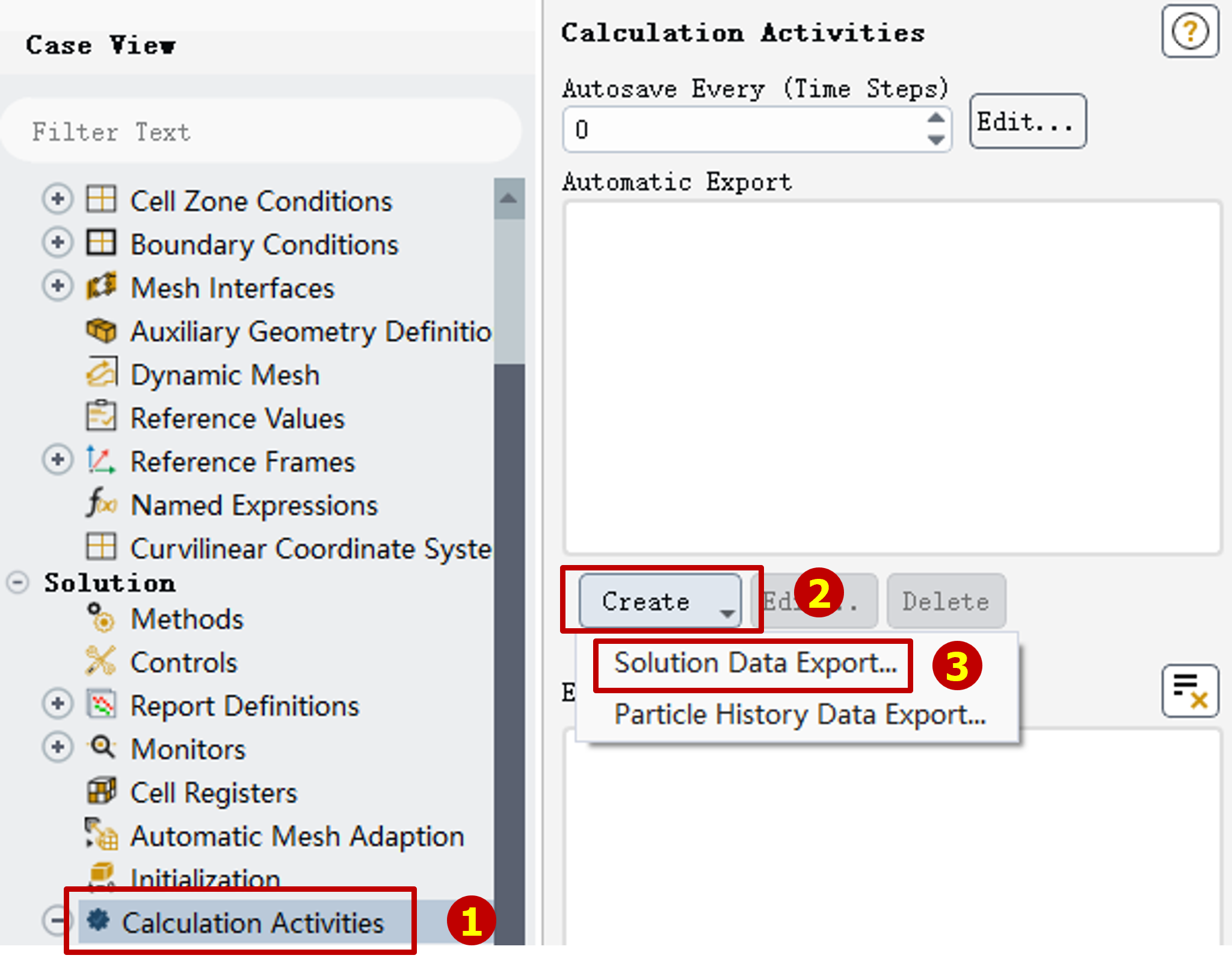
Then double click the "Calculation Activities" in the "Outline view", the "Task Page" will change.
Click the "Create" button then click "Solution Data Export" to set automatic data export.
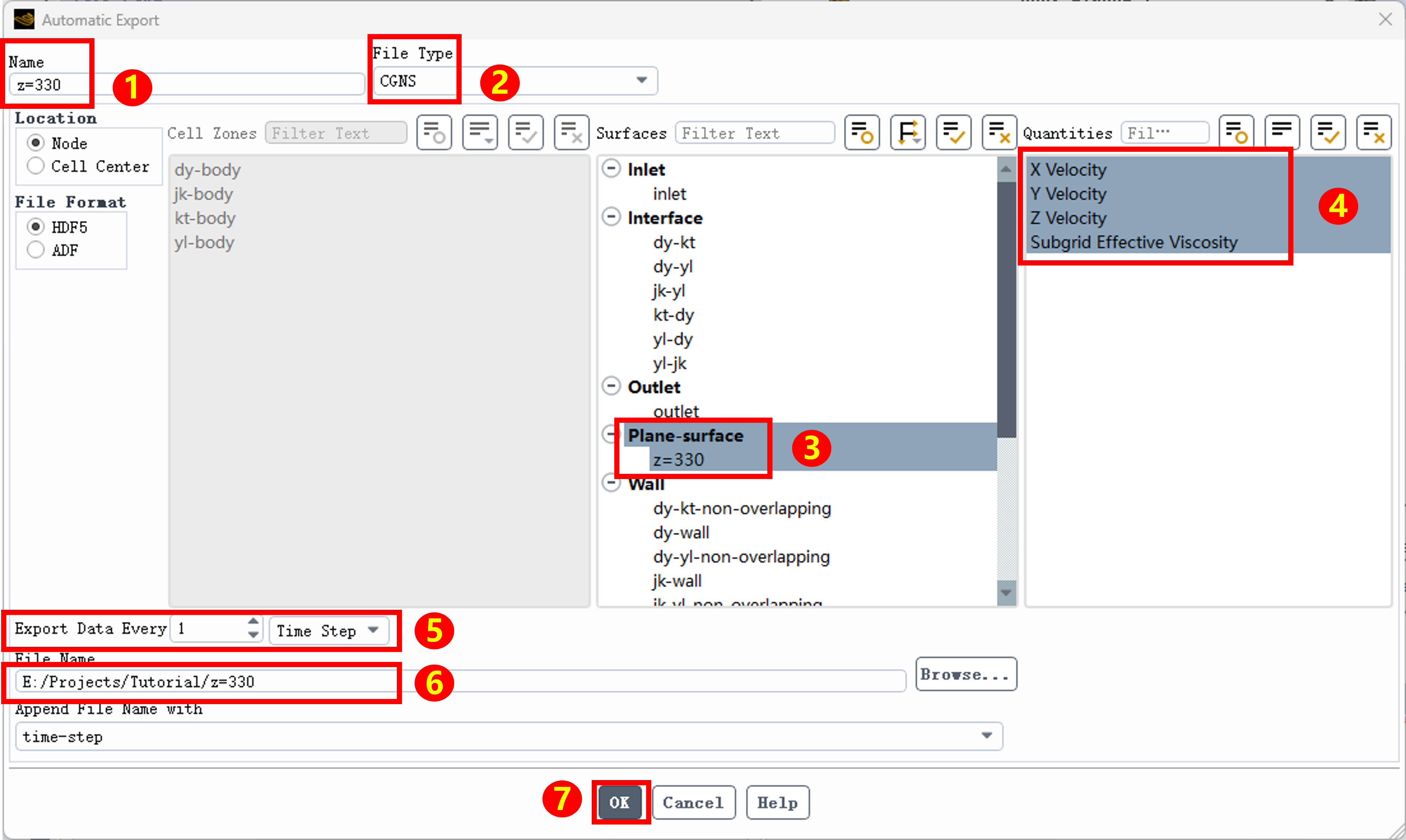
Change the name in the jumped-out window and select "File type" as "CGNS", then select the Iso-surface we just created.
Different from that in doing high-dimensional FFT, we need far more types of data not just "Static Pressure". In entropy production calculation we need these varibles:
- Velocity component X
- Velocity component Y
- Velocity component Z
- SGS Effective Viscosity
Then we need to setup the Automatic Data Export, you can just follow the diagram below to do it.
After doing this, you can start calculation right away and wait for the data.
Oh, do not for get setup saving case and data automatically, you don't wanna lose your data by accident, right?
Step 2. Data processing.
After quite a long wait, we’ve finally gathered all the data needed for our entropy production analysis. 🎉🎉🎉Without further ado, let’s jump straight into the next stage: data processing.
Before we start, a small but important heads-up ⚠️: this step involves computing partial derivatives over a large volume of data. As a result, it can be rather demanding on your computer—especially in terms of CPU performance and disk I/O.
To keep things running smoothly (and to avoid watching your progress bar crawl at a glacial pace 🐢), I strongly recommend using a machine with a high-performance CPU (for example, an i5-12400 or better) and storing all data on an SSD. Otherwise, I/O bottlenecks may significantly slow down the entire data-processing workflow.
First we gonna do is convert data format from CGNS into DAT. The process is the same as I ve introduced in "How to do high-dimensional FFT with Fluent data?" So, you can follow that tutorial to get this job done.
According to the entropy production formula, the total value consists of direct and turbulent components. This necessitates obtaining two vital variables: the mean velocity and the fluctuating velocity at each mesh node. These two data points are the keys to calculating entropy production.
To save you some time, I’ve made my MATLAB code available for everyone to use. Feel free to download through this link.
After processing the data files through the program, the header text must be replaced to match the processed data. This step ensures that Tecplot correctly identifies the data structure and prevents errors caused by mismatches between the data columns and their respective variable names. create a new text document. Then, open any of the recently processed .DAT files using Notepad (Text Editor). You will find the header text structured as follows:
TITLE = "Tecplot Export"
VARIABLES = "CoordinateX"
"CoordinateY"
"CoordinateZ"
"Fluctuating Vx"
"Fluctuating Vy"
"Fluctuating Vz"
"AVG Vx"
"AVG Vy"
"AVG Vz"
"SGS_Viscosity_Eff"
ZONE T="Entropy Zone"
 STRANDID=1, SOLUTIONTIME=0
 Nodes="Node count of your data", Faces="Face count of your data", Elements="Element count of your data", ZONETYPE=FEPolygon
 DATAPACKING=BLOCK
 NumConnectedBoundaryFaces=0, TotalNumBoundaryConnections=0
 AUXDATA Time="0"
 DT=(SINGLE SINGLE SINGLE SINGLE SINGLE SINGLE SINGLE SINGLE SINGLE SINGLE)
To give you a visual reference, the header from the example data is shown below. Your task is to swap all variable names after VARIABLES with my list. Then, adjust the count of SINGLE (or DOUBLE) values in the DT section to correspond with the number of variables.
Note: a space must be included before the closing parenthesis.
Please note that this is for reference only. Data header formats may vary depending on your specific case; avoid copying and pasting the entire block blindly.
After doing this, 50% of this tutorial has been done.
Step 3. Calculationg Entropy By Using Tecplot.
Next we gonna do is calculating the entropy production by using tecplot.
First, you need a loop code like I metioned in the tutorial of high dimensional FFT:"How to do high-dimensional FFT with Fluent data?"
Then, You need these expressions down below to calculate:
{Total_Temperature}=300
{Direct_Entropy}=2*{SGS_Viscosity_Eff}/{Total_Temperature}*((ddx({AVG Vx}))**2+(ddy({AVG Vy}))**2+(ddz({AVG Vz}))**2)+{SGS_Viscosity_Eff}/{Total_Temperature}*((ddy({AVG Vx})+ddx({AVG Vy}))**2+(ddz({AVG Vx})+ddx({AVG Vz}))**2+(ddz({AVG Vy})+ddy({AVG Vz}))**2)
{Turbulent_Entropy}=2*{SGS_Viscosity_Eff}/{Total_Temperature}*((ddx({Fluctuating Vx}))**2+(ddy({Fluctuating Vy}))**2+(ddz({Fluctuating Vz}))**2)+{SGS_Viscosity_Eff}/300*((ddy({Fluctuating Vx})+ddx({Fluctuating Vy}))**2+(ddz({Fluctuating Vx})+ddx({Fluctuating Vz}))**2+(ddz({Fluctuating Vy})+ddy({Fluctuating Vz}))**2)
{Total_Entropy}={Direct_Entropy}+{Turbulent_Entropy}
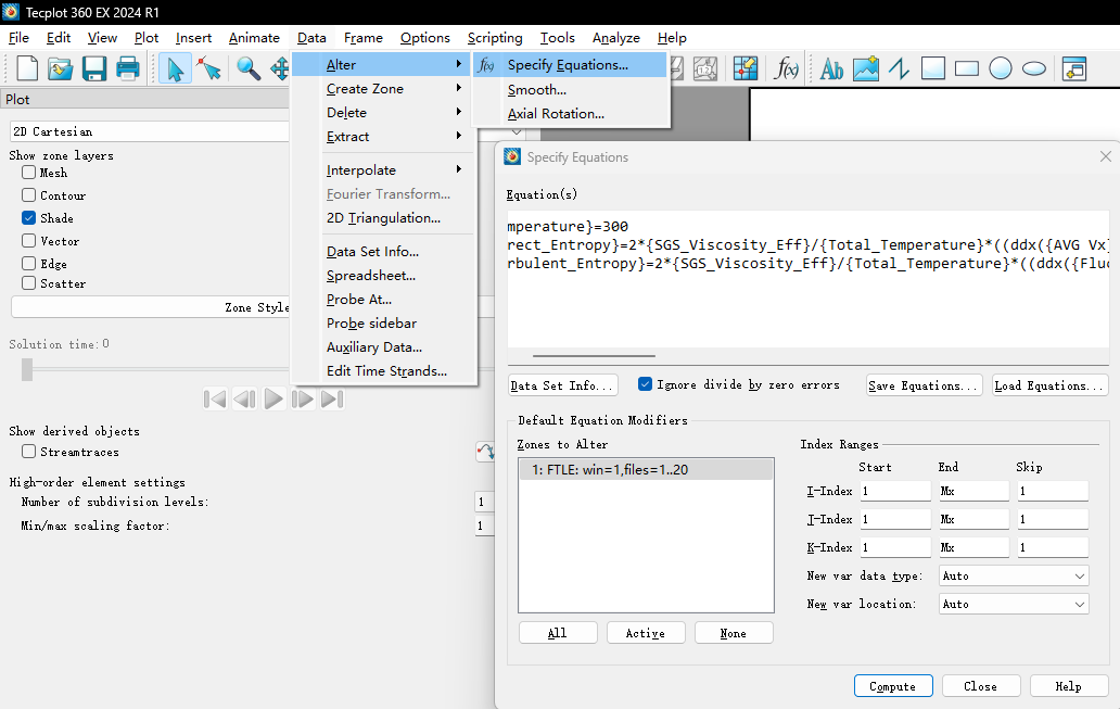
Then press "Compute", you will get the result of entropy production.